


This repo contains the ClustAssess R package, which provides a set of tools for evaluating clustering robustness.
Please check the ClustAssessPy module for a Python implementation of the ClustAssess package.
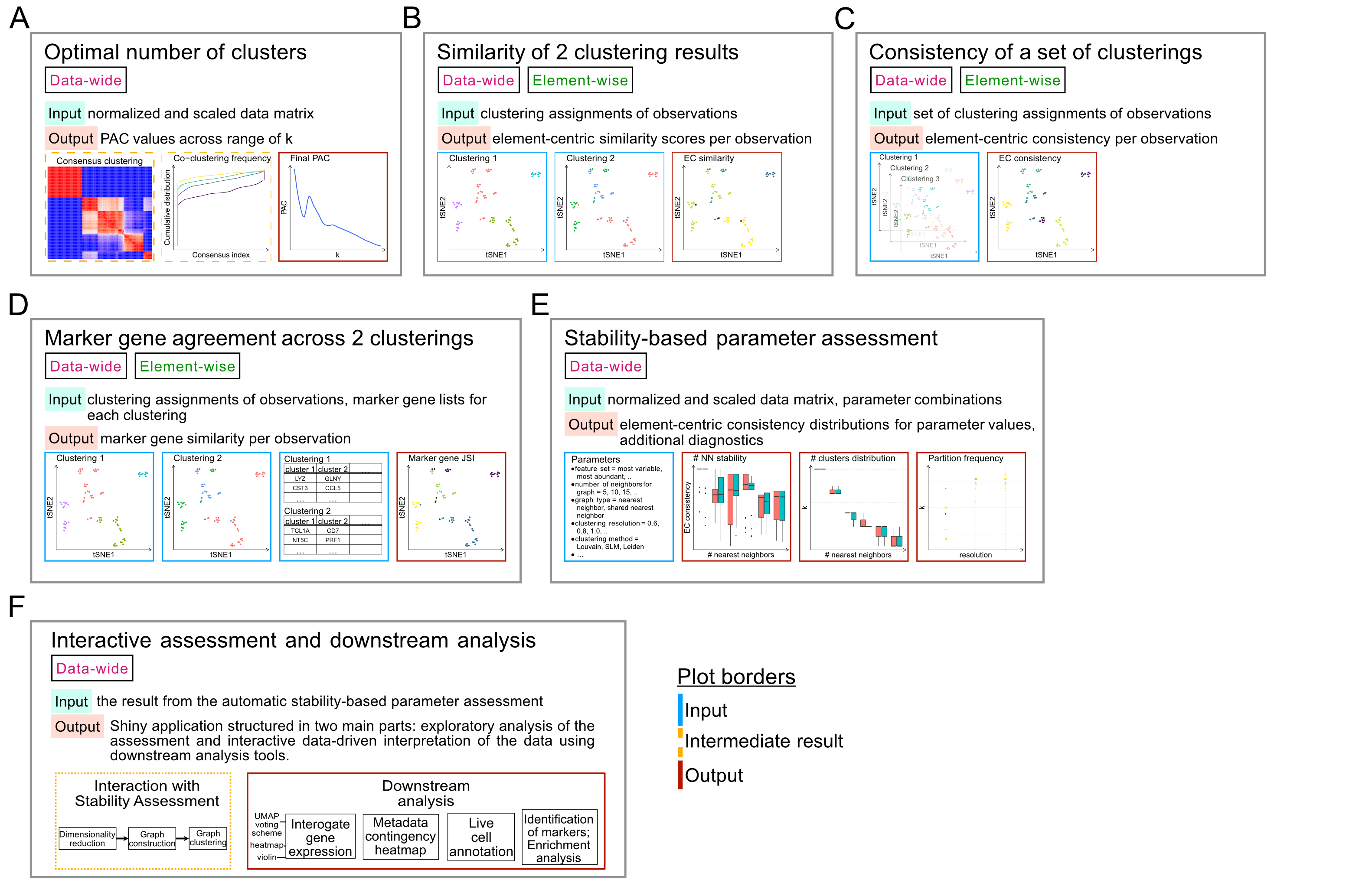
To assess clustering robustness, the proportion of ambiguously clustered pairs (PAC) [1] uses a consensus clustering. The rate of element co-clustering is recorded across various numbers of clusters, k. The lower the PAC, the stabler the clustering for that k.
ClustAssess uses a heirarchical clustering as base for the consensus clustering, and an optimized Rcpp [2] implementation to compute the PAC values. To calculate PAC, we write:
cc_res = consensus_cluster(your_data, n_reps=50, k_max=20, p_sample=0.8, p_feature=0.8)
It is important that the PAC has converged before using it to assess
your data; the pac_convergence function can be used to
visualize the PAC curves across iterations:
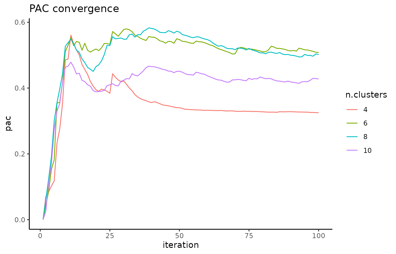
As the curves have evened out, we surmize that PAC has converged in
this case. If the PAC has not converged, increase the
n_reps value.
If the dataset contains >1000 elements, we recommend calculating a geometric sketch [3] of your data of size <1000, and running PAC on that sketch.
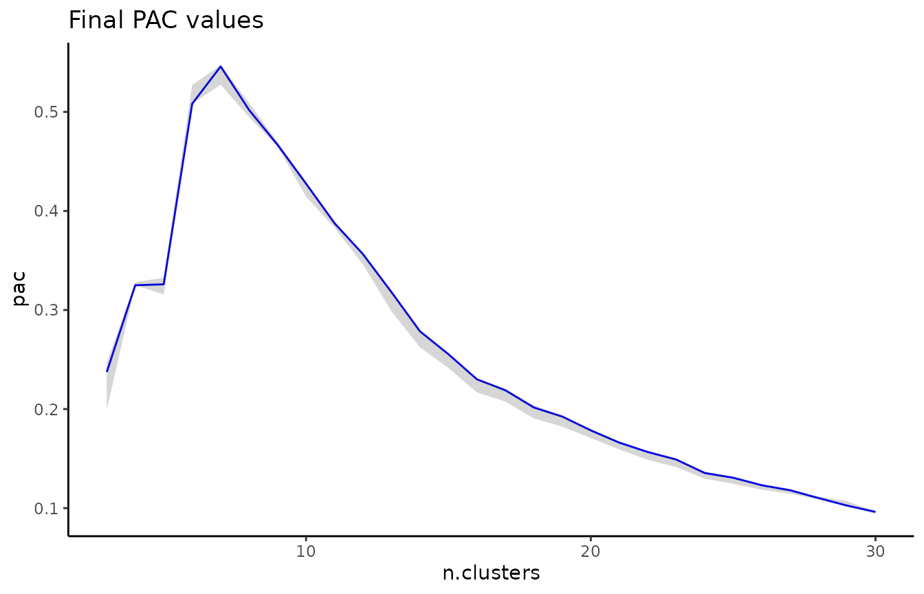
A local minimum in the PAC landscape, as visualized below using the
pac_landscape function, can be interpreted as an optimal
k for the dataset:
Element-centric similarity (ECS) [4] is a per-observation measure of clustering similarity. Briefly, ECS is obtained by constructing a cluster-induced element graph, and subsequently calculating the stationary probability distribution of a random walk with restarts (also known as a personalized Pagerank) over the elements.
In addition to providing per-element information on clustering agreement, ECS avoids several pitfalls associated with other measures of clustering similarity (refer to [4] for more detail).
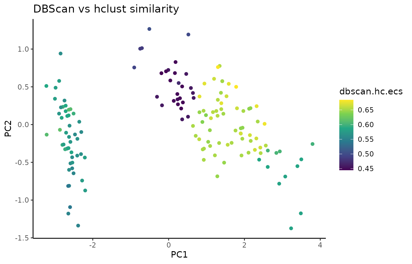
To compare two clusterings with ECS, we use the
element_sim_elscore function:
ecs = element_sim_elscore(clustering_result1, clustering_result2, alpha=0.9)
where 1-alpha is the restart probability of the random
walk. We can subsequently visualize the ECS on a PCA of the data:
In addition to flat disjoint clusterings (like the result of k-means
for example), ClustAssess can also compare overlapping clusterings and
hierarchical clusterings; refer to the
comparing-soft-and-hierarchical vignette for more
detail.
Besides comparing two clusterings with
element_sim_elscore, ClustAssess also enables computing the
per-element consistency (aka frustration) between a set of clusterings
with the element_consistency function, and comparing a set
of clusterings with a ground truth partitioning of elements with the
element_agreement function.
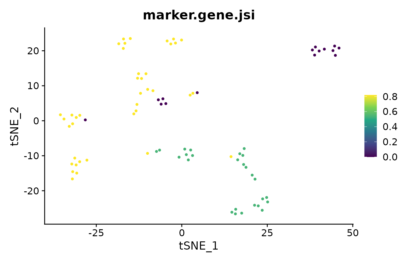
In the analysis of single-cell RNA-seq data, cluster marker genes are
typically used to infer the cell type of clusters. However, two
different clustering results may lead to two different sets of markers
for the cells. The marker_overlap function allows the
comparison of two sets of markers. The output can be either as the
number of common marker genes per cell, or as Jaccard similarity (size
of intersect divided by size of union) per cell.
The most common clustering pipeline for single-cell data consists of
constructing a nearest-neighbor graph of the cells, followed by
community detection to obtain the clustering. This pipeline is available
in multiple single-cell toolkits, including Seurat, Monocle v3, and
SCANPY. ClustAssess provides several methods to assess the stability of
parameter choices that influence the final clustering, for example to
evaluate feature sets, we use get_feature_stability_object,
and plot the results with
plot_feature_stability_boxplot:
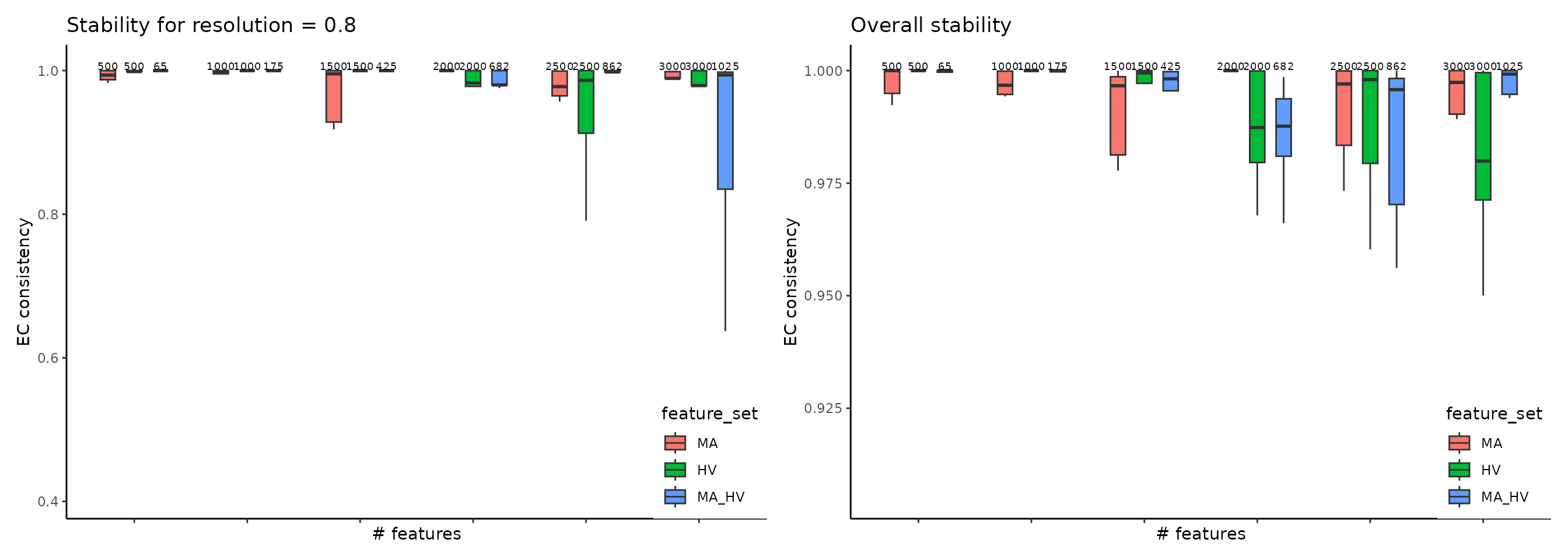
where the higher element-centric consistency (ECC) indicates more stable clustering results across random seeds. For more details, please see this vignette.
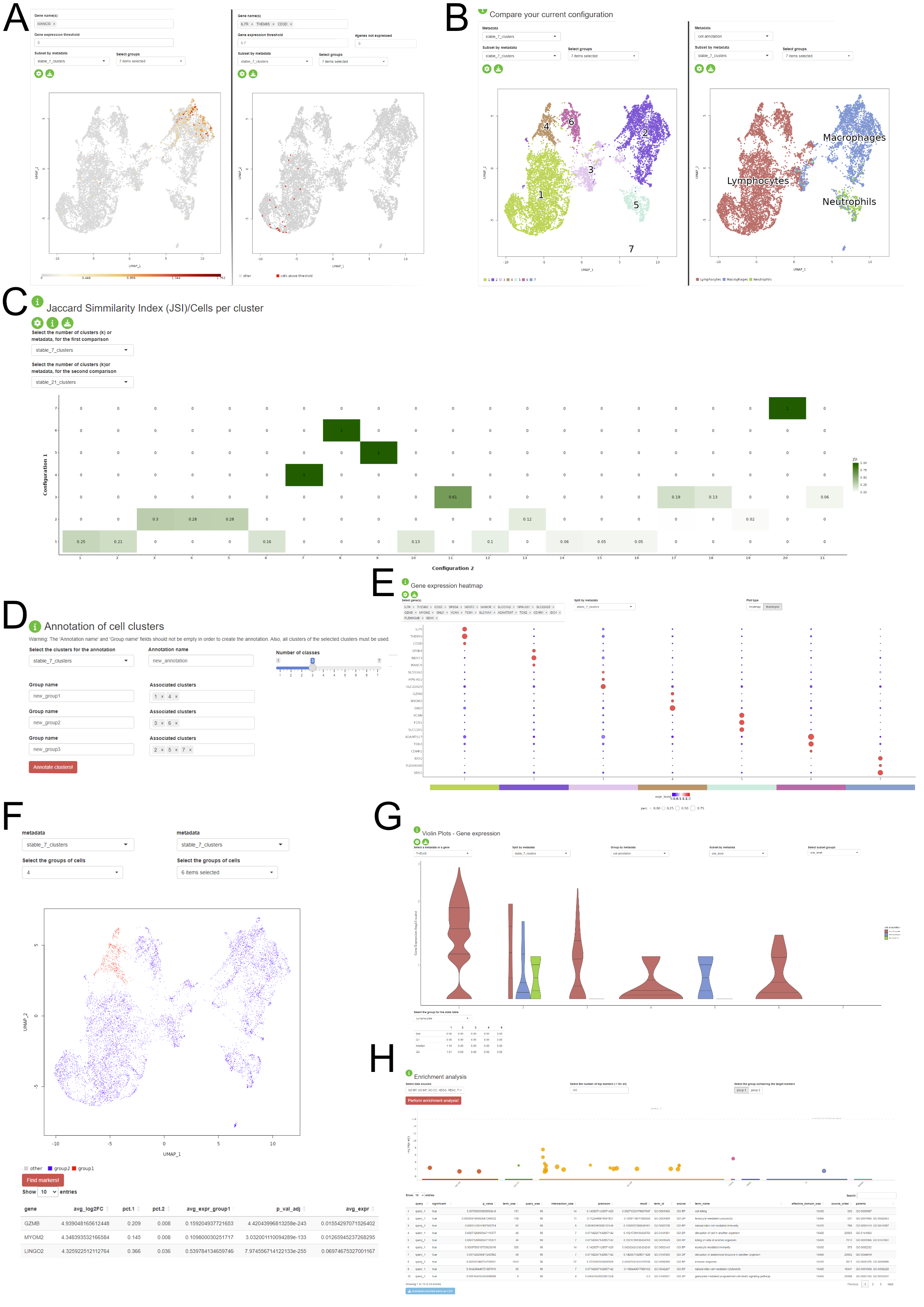
Another feature of the package consists in providing a Shiny application where the user can interactively visualize the stability assessment of the clustering and perform some downstream analysis steps on the dataset without prior R knwoledge. The application is divided into three major components: - Stability Assessments: the user is presented with the assessment of the clustering stability for each of the three steps of the PhenoGraph pipeline. This component is structured in three tabs, one for each step. The user is prompted to select the stable configurations in order to proceed to the next section. - Comparison of configuration and downstream analysis: the user can visually assess the clustering results and the pattern on expression based on the variety of visualisations provided in this section, which contains UMAP plots (A - one or multiple gene expression, B - metadata distribution), violin and boxplots (G), gene expression pseudobulk heatmap and bubbleplots (E), metadata association heatmaps (C). The biological interpretation is enhanced by the possibility of identifying the marker genes for each cluster (F) and the enrichment analysis of the detected differentially expressed genes (H). The app allows custom annotation of the clusters and the already existing metadata (D). - Sandbox: this tab provides more flexibility for the user in temrs of the selected configuration. This approach is available, but not encouraged, as the results might not be stable and reproducible. This tab also contains elements such as panels for changing the colourscheme of the figures.
The application can be generated using the output of the
automatic_stability_assessment function and a normalised
expression matrix.
If your dataset is large, the runtime for the tools described above may be prohibitive. In these cases, we recommend subsampling your data using geometric sketching [3]. In R, the subsampling can be done via reticulate:
geosketch <- reticulate::import('geosketch')
assuming data.embed contains a dimensionality reduction of your data, you can then call:
sketch.indices <- geosketch$gs(data.embed, sketch.size, one_indexed = TRUE)
and use the resulting indices for your subsample. For PAC, subsampling to <1000 cells should help, and for ECS and data assessment functions, <5000 cells may be appropriate (and parallelization can further help reduce the runtime).
ClustAssess can be installed from CRAN:
install.packages("ClustAssess")
or from github using remotes:
remotes::install_github("Core-Bioinformatics/ClustAssess")
The following packages are required for ClustAssess:
To use all stability-based assessment methods, and run all examples and vignettes, the following packages are also needed:
To manually install the required dependencies, please use the following commands:
install.packages(c("dplyr", "DT", "fastcluster", "foreach", "glue", "Gmedian", "ggnewscale", "ggplot2", "ggrastr", "ggrepel", "ggtext", "gprofiler2", "igraph", "jsonlite", "leiden", "Matrix", "matrixStats", "methods", "progress", "stringr", "paletteer", "plotly", "qualpalr", "RANN", "reshape2", "rlang", "Seurat", "shiny", "shinyjs", "shinyLP", "shinyWidgets", "stats", "uwot", "vioplot"), Ncpus = 1)
install.packages("BiocManager")
BiocManager::install(c("ComplexHeatmap"))
To manually install the suggested dependencies, please use the following commands:
install.packages(c("colourpicker", "devtools", "doParallel", "doRNG", "knitr", "leidenbase", "patchwork", "ragg", "rmarkdown", "RhpcBLASctl", "scales", "SeuratObject", "styler", "testthat"), Ncpus = 1)

install.packages("BiocManager")
BiocManager::install(c("DelayedMatrixStats", "rhdf5"))

devtools::install_github('cole-trapnell-lab/monocle3')
devtools::install_github("Jiefei-Wang/SharedObject")
To manually install the packages that are exclusively used to build the vignettes, please use the following commands:
devtools::install_github('satijalab/seurat-data')
install.packages(c("harmony", "Signac"))
BiocManager::install("Rsamtools")Note: The package is under active development, and the release branches might contain additional features and bug fixes.
If you have used ClustAssess in your work, please cite Shahsavari et al. 2022:
Shahsavari, A., Munteanu, A., & Mohorianu, I. (2022). ClustAssess: Tools for Assessing the Robustness of Single-Cell Clustering. bioRxiv. https://doi.org/10.1101/2022.01.31.478592or in BibTex:
@ARTICLE{clustassess,
  title     = "ClustAssess: Tools for Assessing the Robustness of Single-Cell Clustering",
  author    = "Shahsavari, Arash and Munteanu, Andi and Mohorianu, Irina",
  journal   = "bioRxiv",
  year      =  2022,
  url       = "https://doi.org/10.1101/2022.01.31.478592",
  language  = "en"
}[1] Șenbabaoğlu, Y., Michailidis, G., & Li, J. Z. (2014). Critical limitations of consensus clustering in class discovery. Scientific reports, 4(1), 1-13. https://doi.org/10.1038/srep06207
[2] Eddelbuettel, D., & Balamuta, J. J. (2018). Extending R with C++: A brief introduction to Rcpp. The American Statistician, 72(1), 28-36. https://doi.org/10.1080/00031305.2017.1375990
[3] Hie, B., Cho, H., DeMeo, B., Bryson, B., & Berger, B. (2019). Geometric sketching compactly summarizes the single-cell transcriptomic landscape. Cell systems, 8(6), 483-493. https://doi.org/10.1016/j.cels.2019.05.003
[4] Gates, A. J., Wood, I. B., Hetrick, W. P., & Ahn, Y. Y. (2019). Element-centric clustering comparison unifies overlaps and hierarchy. Scientific reports, 9(1), 1-13. https://doi.org/10.1038/s41598-019-44892-y