Functions for the determination of similarity of highly variable dissolution profiles of two drug formulations are provided. Estimation of f1, f2 and bootstrap f2 is implemented. In addition, functions following the model-independent MCR (multivariate confidence region) procedure and the T2-test for equivalence procedure are available.
A stable version of disprofas can be installed from
CRAN:
install.packages("disprofas")The development version is available from GitHub by:
# install.packages("devtools")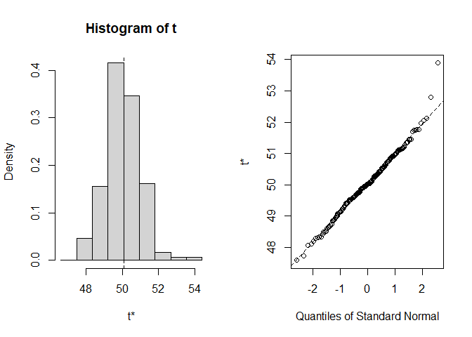
# devtools::install_github("piusdahinden/disprofas")Example 1 illustrates how to solve a common problem by aid of the bootstrap f2 procedure proposed by Shah et al. (1998) using a data set containing the dissolution data of one reference batch and one test batch of n = 12 tablets each, i.e. the dissolution profiles of the % drug release observed at 0, 30, 60, 90 and 180 minutes (See Shah et al. (1998), Table 4).
library(disprofas)

# Data frame
str(dip2)
#> 'data.frame':    72 obs. of  8 variables:
#>  $ type  : Factor w/ 2 levels "Reference","Test": 1 1 1 1 1 1 1 1 1 1 ...
#>  $ tablet: Factor w/ 12 levels "1","2","3","4",..: 1 2 3 4 5 6 7 8 9 10 ...
#>  $ batch : Factor w/ 6 levels "b0","b1","b2",..: 1 1 1 1 1 1 1 1 1 1 ...
#>  $ t.0   : int  0 0 0 0 0 0 0 0 0 0 ...
#>  $ t.30  : num  36.1 33 35.7 32.1 36.1 34.1 32.4 39.6 34.5 38 ...
#>  $ t.60  : num  58.6 59.5 62.3 62.3 53.6 63.2 61.3 61.8 58 59.2 ...
#>  $ t.90  : num  80 80.8 83 81.3 72.6 83 80 80.4 76.9 79.3 ...
#>  $ t.180 : num  93.3 95.7 97.1 92.8 88.8 97.4 96.8 98.6 93.3 94 ...
# Perform estimation and print a summary
res1 <- bootstrap_f2(data = dip2[dip2$batch %in% c("b0", "b4"), ],
                         tcol = 5:8, grouping = "batch",
                         rr = 200, new_seed = 421, use_ema = "no")

class(res1)
#> [1] "bootstrap_f2"summary(res1)
#>
#> STRATIFIED BOOTSTRAP
#>
#>
#> Call:
#> boot(data = data, statistic = get_f2, R = rr, strata = data[,
#> grouping], grouping = grouping, tcol = tcol[ok])
#>
#>
#> Bootstrap Statistics :
#> original bias std. error
#> t1* 50.07187 -0.02553234 0.9488015
#>
#>
#> BOOTSTRAP CONFIDENCE INTERVAL CALCULATIONS
#> Based on 200 bootstrap replicates
#>
#> CALL :
#> boot.ci(boot.out = t_boot, conf = confid, type = "all", L = jack$loo.values)
#>
#> Intervals :
#> Level Normal Basic
#> 90% (48.54, 51.66 ) (48.46, 51.71 )
#>
#> Level Percentile BCa
#> 90% (48.43, 51.68 ) (48.69, 51.99 )
#> Calculations and Intervals on Original Scale
#> Some BCa intervals may be unstable
#>
#>
#> Shah's lower 90% BCa confidence interval:
#> 48.64613
# Prepare a graphical representation
plot(res1)
#>
#> Shah's lower 90% BCa confidence interval:
#>  48.64613
Example 2 illustrates how to solve a common problem by aid of the model-independent non-parametric multivariate confidence region (MCR) procedure proposed by Tsong et al. (1996) using a data set containing the dissolution data of one reference batch and one test batch of n = 6 tablets each, i.e. the dissolution profiles of the % drug release observed at 5, 10, 15, 20, 30, 60, 90 and 120 minutes (see Tsong et al. (1996), Table 1).
library(disprofas)

# Data frame
str(dip3)
#> 'data.frame':    24 obs. of  6 variables:
#>  $ cap  : Factor w/ 12 levels "1","2","3","4",..: 1 2 3 4 5 6 7 8 9 10 ...
#>  $ batch: Factor w/ 2 levels "blue","white": 2 2 2 2 2 2 2 2 2 2 ...
#>  $ type : Factor w/ 2 levels "ref","test": 1 1 1 1 1 1 1 1 1 1 ...
#>  $ x.15 : num  49 15 56 57 6 62 23 11 9 42 ...
#>  $ x.20 : num  86 59 84 87 58 90 71 64 61 81 ...
#>  $ x.25 : num  98 96 96 99 90 97 97 92 88 96 ...
# Perform estimation and print a summary
res2 <- mimcr(data = dip3, tcol = 4:6, grouping = "batch")

class(res2)
#> [1] "mimcr"summary(res2)
#>
#> Results of Model-Independent Multivariate Confidence Region (MIMCR)
#> approach to assess equivalence of highly variable in-vitro
#> dissolution profiles of two drug product formulations
#>
#> Did the Newton-Raphson search converge? Yes
#> Are the points located on the confidence region boundary (CRB)? Yes
#>
#> Parameters (general):
#> Significance level: 0.05
#> Degrees of freedom (1): 3
#> Degrees of freedom (2): 20
#> Mahalanobis distance (MD): 0.2384
#> (F) scaling factor K: 1.818
#> (MD) scaling factor k: 6
#> Hotelling's T2: 0.341
#>
#> Parameters specific for Tsong (1996) approach:
#> Maximum tolerable average difference: 10
#> Similarity limit: 2.248
#> Observed upper limit: 1.544
#>
#> Parameters specific for Hoffelder (2016) approach:
#> Noncentrality parameter: 30.32
#> Critial F (Hoffelder): 4.899
#> Probability p (Hoffelder): 2.891e-08
#>
#> Conclusions:
#> Tsong (1996): Similar
#> Hoffelder (2016): SimilarExample 3 illustrates how to solve a common problem by aid
of the T2-test for equivalence procedure proposed by
Hoffelder (2016) using a data set containing the dissolution data of one
reference batch and one test batch of n = 12 capsules each,
i.e. the dissolution profiles of the % drug release observed at 15, 20
and 25 minutes (see Hoffelder (2016), Figure 1 (data not shown in
publication, but the data set is available on CRAN, package T2EQ, data set
ex_data_pharmind)).
library(disprofas)

# Data frame
str(dip4)
#> 'data.frame':    24 obs. of  4 variables:
#>  $ type: Factor w/ 2 levels "ref","test": 1 1 1 1 1 1 1 1 1 1 ...
#>  $ x.10: num  30 10 32 50 16 17 47 37 41 42 ...
#>  $ x.20: num  76 59 77 90 64 77 87 83 82 78 ...
#>  $ x.30: num  97 96 97 98 95 96 98 98 98 98 ...
# Perform estimation and print a summary
res3 <- mimcr(data = dip4, tcol = 2:4, grouping = "type")
summary(res3)
#>
#> Results of Model-Independent Multivariate Confidence Region (MIMCR)
#> approach to assess equivalence of highly variable in-vitro
#> dissolution profiles of two drug product formulations
#>
#> Did the Newton-Raphson search converge? Yes
#> Are the points located on the confidence region boundary (CRB)? Yes
#>
#> Parameters (general):
#> Significance level:                   0.05
#> Degrees of freedom (1):               3
#> Degrees of freedom (2):               20
#> Mahalanobis distance (MD):            2.824
#> (F) scaling factor K:                 1.818
#> (MD) scaling factor k:                6
#> Hotelling's T2:                       47.85
#>
#> Parameters specific for Tsong (1996) approach:
#> Maximum tolerable average difference: 10
#> Similarity limit:                     17.18
#> Observed upper limit:                 4.129
#>
#> Parameters specific for Hoffelder (2016) approach:
#> Noncentrality parameter:              1770
#> Critial F (Hoffelder):                373.5
#> Probability p (Hoffelder):            8.428e-110
#>
#> Conclusions:
#>       Tsong (1996):  Similar
#>   Hoffelder (2016):  Similar
Example 4 illustrates the tolerance interval approach proposed by Martinez & Zhao (2018) using the data set that was used in Example 1. In the graphical representation of the data, the data points of the reference batch are shown as grey dots (●), the data points of the test batch as red crosses (✕), the average time course is shown as blue line and the associated tolerance interval limits (TL) as green, orange and red lines that are drawn at TL, TL ± S1 (5%) and TL ± S2 (15%), respectively.
library(disprofas)

# Data frame
str(dip1)
#> 'data.frame':    12 obs. of  10 variables:
#>  $ type  : Factor w/ 2 levels "R","T": 1 1 1 1 1 1 2 2 2 2 ...
#>  $ tablet: Factor w/ 6 levels "1","2","3","4",..: 1 2 3 4 5 6 1 2 3 4 ...
#>  $ t.5   : num  42.1 44.2 45.6 48.5 50.5 ...
#>  $ t.10  : num  59.9 60.2 55.8 60.4 61.8 ...
#>  $ t.15  : num  65.6 67.2 65.6 66.5 69.1 ...
#>  $ t.20  : num  71.8 70.8 70.5 73.1 72.8 ...
#>  $ t.30  : num  77.8 76.1 76.9 78.5 79 ...
#>  $ t.60  : num  85.7 83.3 83.9 85 86.9 ...
#>  $ t.90  : num  93.1 88 86.8 88 89.7 ...
#>  $ t.120 : num  94.2 89.6 90.1 93.4 90.8 ...
# Perform estimation and print a summary
res4 <- mztia(data = dip1, shape = "wide", tcol = 3:10, grouping = "type",
                reference = "R")

class(res4)
#> [1] "mztia"summary(res4)
#>
#> Results of Martinez & Zhao Tolerance Interval (TI) Approach
#> (TI limits calculated at each time point of the dissolution profiles of a set of reference batches)
#>
#> Time Mean LTL UTL S1.LTL S1.UTL S2.LTL S2.UTL
#> 1 5 46.77167 27.22641 66.31693 22.22641 71.31693 12.22641 81.31693
#> 2 10 60.13333 46.15483 74.11184 41.15483 79.11184 31.15483 89.11184
#> 3 15 67.27500 56.90417 77.64583 51.90417 82.64583 41.90417 92.64583
#> 4 20 71.98667 65.44354 78.52979 60.44354 83.52979 50.44354 93.52979
#> 5 30 78.07000 69.54259 86.59741 64.54259 91.59741 54.54259 101.59741
#> 6 60 84.81667 77.20275 92.43058 72.20275 97.43058 62.20275 107.43058
#> 7 90 89.09333 76.24588 100.00000 71.24588 105.00000 61.24588 115.00000
#> 8 120 91.43833 80.29321 100.00000 75.29321 105.00000 65.29321 115.00000
#>
#> Abbreviations:
#> TL: Tolerance Interval Limit (TL); LTL: lower TL; UTL: upper TL; S1: level 1 boundary (LTL - ) or (UTL + ); S2: level 2 boundary (LTL - ) or (UTL + ).
# Prepare a graphical representation
ggres4 <- plot_mztia(res4)
class(ggres4)
#> [1] "plot_mztia"plot(ggres4)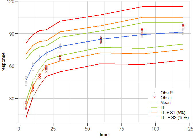
Example 5 illustrates how to solve a common problem by aid of the model-dependent approach as proposed by Sathe, Tsong & Shah (1996) or by Tsong, Hammerstrom & Chen (1997).
In Example 5a, the data set shown in Table 4 of Tsong, Hammerstrom & Chen (1997) is used which contains the Weibull parameter estimates obtained from fitting of Weibull curves to the cumulative dissolution profiles of individual tablets of three reference batches and one test batch of n = 12 tablets each. First, a one-sample T2-test is performed with the Weibull parameters of the reference group only, followed by a two-sample T2-test to compare the Weibull parameters of the reference batches withe the Weibull parameters of the test batch.
library(disprofas)

str(dip7)
#> 'data.frame':    48 obs. of  5 variables:
#>  $ tablet: Factor w/ 12 levels "1","2","3","4",..: 1 2 3 4 5 6 7 8 9 10 ...
#>  $ batch : Factor w/ 4 levels "b1","b2","b3",..: 1 1 1 1 1 1 1 1 1 1 ...
#>  $ type  : Factor w/ 2 levels "ref","test": 1 1 1 1 1 1 1 1 1 1 ...
#>  $ alpha : num  0.583 0.496 0.571 0.579 0.593 ...
#>  $ beta  : num  0.555 0.655 0.489 0.588 0.485 ...
t_param <- c("alpha", "beta")
# One-sample T2 test with only the reference data
res1 <- get_T2_one(m = as.matrix(dip7[dip7$type == "ref", t_param]),
mu = colMeans(as.matrix(dip7[dip7$type == "test", t_param])),
signif = 0.05)
# Two-sample T2 test comparing the reference with the test data
res2 <- get_T2_two(m1 = as.matrix(dip7[dip7$type == "ref", t_param]),
m2 = as.matrix(dip7[dip7$type == "test", t_param]),
signif = 0.05)
# Estimates
res1$Parameters
#> dm df1 df2 signif K k T2
#> 3.027907 2.000000 34.000000 0.050000 17.485714 36.000000 330.055950
#> F F.crit t.crit p.F
#> 160.312890 3.275898 2.341969 0.000000res2$Parameters
#> dm df1 df2 signif K k
#> 3.247275e+00 2.000000e+00 4.500000e+01 5.000000e-02 4.402174e+00 9.000000e+00
#> T2 F F.crit t.crit p.F
#> 9.490313e+01 4.642001e+01 3.204317e+00 2.317152e+00 1.151701e-11Since in the current example we have a two-dimensional situation, the results can be illustrated graphically. Based on the reference batch parameter estimates, a (1 − signif)100% confidence region (CR) can be constructed. All points on this CR have the same Mahalanobis distance. This distance sets the upper confidence limit (UCL).
# Stretch factor
qfk <- as.numeric(sqrt(res2$Parameters["k"] / res2$Parameters["K"] *
                         res2$Parameters["F.crit"]))

# Cholesky decomposition, scaling and centering of confidence region
RR         <- chol(res2$covs$S.b1) # chol(res1$cov)
angles     <- seq(0, 2 * pi, length.out = 200)
ellipse    <- qfk[1] * cbind(cos(angles), sin(angles)) %*% RR
ellipseCtr <- sweep(ellipse, 2, res2$means$mean.b1, "+")

# Determination of ucl
ucl <- mahalanobis(x = ellipseCtr[1, ],
                   center = res2$means$mean.b1, cov = res2$covs$S.b1)
The UCL allows checking which points lie outside the CR and which points lie inside.
# Determination of scores
scores <- c(mahalanobis(x = as.matrix(dip7[dip7$type == "ref", t_param]),
                        center = res2$means$mean.b1,
                        cov = res2$covs$S.b1),
            mahalanobis(x = as.matrix(dip7[dip7$type == "test", t_param]),
                        center = res2$means$mean.b1,
                        cov = res2$covs$S.b1))

# Check if scores are greater than ucl
is_out <- scores > ucl

# Points in the dip7 data frame lying outside the confidence region
dip7[is_out, ]
#>    tablet batch type   alpha    beta
#> 9       9    b1  ref 0.46120 0.47234
#> 16      4    b2  ref 0.44647 0.71136
#> 21      9    b2  ref 0.43405 0.49848
#> 28      4    b3  ref 0.40571 0.74920
#> 33      9    b3  ref 0.46120 0.47234
#> 37      1    b4 test 0.38827 0.75826
#> 38      2    b4 test 0.42679 0.75668
#> 39      3    b4 test 0.43043 0.70732
#> 42      6    b4 test 0.43187 0.82644
#> 45      9    b4 test 0.39666 0.82681
#> 46     10    b4 test 0.42297 0.76226
#> 47     11    b4 test 0.43270 0.78700
#> 48     12    b4 test 0.45036 0.75428
These results are displayed graphically in the following figure. The points of the reference batches are shown as blue circles (◯) and the points of the test batch as red crosses (✕). The CR boundary is shown as blue ellipse. The bold blue diamond (◇) represents the centre point of the ellipse. The points that have been identified to lie outside the CR are highlighted by yellow greek crosses (✛).
op <- par(mar = c(2.5, 2.5, 1.2, 0.5), mgp = c(1.5, 0.5, 0), lwd = 1.5)
{
  plot(dip7[dip7$type == "ref", t_param], asp = 1,
       xlim = c(0.3, 0.8), ylim = c(0.3, 0.8), pch = 1, col = "royalblue",
       xlab = "Weibull Scale Parameter (alpha)",
       ylab = "Weibull Shape Parameter (beta)")
  points(dip7[dip7$type == "test", t_param], pch = 4, col = "red")
  points(res1$means$mean.r[1], res1$means$mean.r[2], pch = 5,
         col = "royalblue", lwd = 2)
  lines(ellipseCtr, col = "royalblue")

  # Highlight the points detected to lie outside the confidence region
  points(dip7[is_out, t_param], pch = 3, col = "gold")
}
In Example 5b, the data set shown in Table III of Sathe, Tsong & Shah (1996) is used which contains the Weibull parameter estimates obtained from fitting of Weibull curves to the cumulative dissolution profiles of individual tablets of one reference batch and one test / post-change batch with a minor modification and a second test / post-change batch with a major modification, n = 12 tablets each. One-sample T2-tests are performed with the Weibull parameters of the reference and the two test groups separatley.
library(disprofas)

str(dip8)
#> 'data.frame':    36 obs. of  4 variables:
#>  $ tablet: Factor w/ 12 levels "1","2","3","4",..: 1 2 3 4 5 6 7 8 9 10 ...
#>  $ type  : Factor w/ 3 levels "major","minor",..: 3 3 3 3 3 3 3 3 3 3 ...
#>  $ alpha : num  1.1 1.02 1.06 1.03 1.53 ...
#>  $ beta  : num  1.27 1.19 1.09 1.09 1.12 ...
d_dat <- dip8
d_dat[, c("alpha", "beta")] <- log(d_dat[, c("alpha", "beta")])
t_param <- c("alpha", "beta")

res1ref <-
  get_T2_one(m = as.matrix(d_dat[d_dat$type == "ref", t_param]),
             mu = colMeans(as.matrix(d_dat[d_dat$type == "ref", t_param])),
             signif = 0.05)
res1min <-
  get_T2_one(m = as.matrix(d_dat[d_dat$type == "minor", t_param]),
             mu = colMeans(as.matrix(d_dat[d_dat$type == "minor", t_param])),
             signif = 0.05)
res1maj <-
  get_T2_one(m = as.matrix(d_dat[d_dat$type == "major", t_param]),
             mu = colMeans(as.matrix(d_dat[d_dat$type == "major", t_param])),
             signif = 0.05)

# Estimates
res1ref$Parameters
#>        dm       df1       df2    signif         K         k        T2         F
#>  0.000000  2.000000 10.000000  0.050000  5.454545 12.000000  0.000000  0.000000
#>    F.crit    t.crit       p.F
#> 4.102821 2.593093 1.000000res1min$Parameters
#> dm df1 df2 signif K k T2 F
#> 0.000000 2.000000 10.000000 0.050000 5.454545 12.000000 0.000000 0.000000
#> F.crit t.crit p.F
#> 4.102821 2.593093 1.000000res1maj$Parameters
#> dm df1 df2 signif K k T2 F
#> 0.000000 2.000000 10.000000 0.050000 5.454545 12.000000 0.000000 0.000000
#> F.crit t.crit p.F
#> 4.102821 2.593093 1.000000Since in the current example we have a two-dimensional situation, the results can be illustrated graphically. Based on the reference batch parameter estimates, a (1 − signif)100% confidence region (CR) or similarity region, as it is called in the article from Sathe, Tsong & Shah (1996), can be constructed. All points on this CR have the same Mahalanobis distance. The distance obtained with the CR of the reference batches sets the upper confidence limit (UCL).
# Stretch factor
qfk <- c(ref = as.numeric(sqrt(res1ref$Parameters["k"] /
                                 res1ref$Parameters["K"] *
                                 res1ref$Parameters["F.crit"])),
         min = as.numeric(sqrt(res1min$Parameters["k"] /
                                 res1min$Parameters["K"] *
                                 res1min$Parameters["F.crit"])),
         maj = as.numeric(sqrt(res1maj$Parameters["k"] /
                                 res1maj$Parameters["K"] *
                                 res1maj$Parameters["F.crit"])))

# Cholesky decomposition, scaling and centering of confidence region
# Cholesky decomposition, scaling and centering of ellipse
RR_ref         <- chol(res1ref$cov)
angles_ref     <- seq(0, 2 * pi, length.out = 200)
ellipse_ref    <- qfk["ref"] * cbind(cos(angles), sin(angles)) %*% RR_ref
ellipseCtr_ref <- sweep(ellipse_ref, 2, res1ref$means$mean.r, "+")

RR_min         <- chol(res1min$cov)
angles_min     <- seq(0, 2 * pi, length.out = 200)
ellipse_min    <- qfk["min"] * cbind(cos(angles), sin(angles)) %*% RR_min
ellipseCtr_min <- sweep(ellipse_min, 2, res1min$means$mean.r, "+")

RR_maj         <- chol(res1maj$cov)
angles_maj     <- seq(0, 2 * pi, length.out = 200)
ellipse_maj    <- qfk["maj"] * cbind(cos(angles), sin(angles)) %*% RR_maj
ellipseCtr_maj <- sweep(ellipse_maj, 2, res1maj$means$mean.r, "+")

# Determination of ucl
ucl <- mahalanobis(x = ellipseCtr_ref[1, ],
                   center = res1ref$means$mean.r, cov = res1ref$cov)
The UCL allows checking which points lie outside the CR and which points lie inside of it.
# Determination of scores
scores <- c(mahalanobis(x = as.matrix(d_dat[d_dat$type == "ref", t_param]),
                        center = res1ref$means$mean.r,
                        cov = res1ref$cov),
            mahalanobis(x = as.matrix(d_dat[d_dat$type == "minor", t_param]),
                        center = res1ref$means$mean.r,
                        cov = res1ref$cov),
            mahalanobis(x = as.matrix(d_dat[d_dat$type == "major", t_param]),
                        center = res1ref$means$mean.r,
                        cov = res1ref$cov))

is_out <- scores > ucl

# Points in the dip8 data frame lying outside the confidence region
d_dat[is_out, ]
#>    tablet  type      alpha      beta
#> 25      1 major -0.3973333 0.4681895
#> 26      2 major -0.2649817 0.4406971
#> 27      3 major -0.3321635 0.4275201
#> 28      4 major -0.1325947 0.3697896
#> 30      6 major -0.1853662 0.3400800
#> 31      7 major -0.1443555 0.3481608
#> 32      8 major -0.1824936 0.3778198
#> 33      9 major -0.2800976 0.3955023
#> 34     10 major -0.1155680 0.3372220
#> 35     11 major -0.1714766 0.3574926
#> 36     12 major -0.2592760 0.4238353
Finally, the results collected above are displayed graphically for illustration. The black rectangle represents the 3 STD Similarity Region as shown in Figure 4 in the article from Sathe, Tsong & Shah (1996). The points of the reference batch are shown as blue circles (◯), the points of the minor modification batch as green crosses (✕) and the points of the major modification batch as magenta crosses (✕). The CR boundaries are shown as ellipses that are coloured according to the corresponding data points. The bold diamonds (◇) coloured according to the corresponding data points represent the centre points of the ellipses. The points that have been identified to lie outside the CR of the reference batch are highlighted by yellow greek crosses (✛).
op <- par(mar = c(2.5, 2.5, 1.2, 0.5), mgp = c(1.5, 0.5, 0), lwd = 1.5)
t_multiple <- 3

{
  plot(d_dat[d_dat$type == "ref", t_param], asp = 1,
       xlim = c(-0.6, 0.6), ylim = c(-0.2, 0.6), pch = 1, col = "blue2",
       xlab = "ln(alpha)", ylab = "ln(beta)")
  points(d_dat[d_dat$type == "minor", t_param], pch = 4, col = "green3")
  points(d_dat[d_dat$type == "major", t_param], pch = 4, col = "magenta2")
  points(res1ref$means$mean.r[1], res1ref$means$mean.r[2], pch = 5,
         col = "blue2", lwd = 2)
  points(res1min$means$mean.r[1], res1min$means$mean.r[2], pch = 5,
         col = "green3", lwd = 2)
  points(res1maj$means$mean.r[1], res1maj$means$mean.r[2], pch = 5,
         col = "magenta2", lwd = 2)
  lines(ellipseCtr_ref, col = "blue3")
  lines(ellipseCtr_min, col = "green3")
  lines(ellipseCtr_maj, col = "magenta2")
  rect(xleft = t_multiple * -sqrt(diag(res1ref$cov))["alpha"] +
         res1ref$means$mean.r["alpha"],
       ybottom = t_multiple * -sqrt(diag(res1ref$cov))["beta"] +
         res1ref$means$mean.r["beta"],
       xright = t_multiple * sqrt(diag(res1ref$cov))["alpha"] +
         res1ref$means$mean.r["alpha"],
       ytop = t_multiple * sqrt(diag(res1ref$cov))["beta"] +
         res1ref$means$mean.r["beta"])

  # Highlight the points detected to lie outside the confidence region
  points(d_dat[is_out, t_param], pch = 3, col = "gold")
}
Pius Dahinden, Tillotts Pharma AG