A clinical prediction model should produce well calibrated
risk predictions, meaning the predicted probabilities should align with
observed outcome rates. There are different levels at which calibration
can be assessed (see https://pubmed.ncbi.nlm.nih.gov/26772608/); this package
focuses on assessing “moderate” calibration via non-linear calibration
curves. pmcalibration implements calibration curves for
binary and (right censored) time-to-event outcomes and calculates
metrics used to assess the correspondence between predicted and observed
outcome probabilities (the ‘integrated calibration index’ or \(ICI\), aka \(E_{avg}\), as well as \(E_{50}\), \(E_{90}\), and \(E_{max}\) - see below).
A goal of pmcalibration is to implement a range of
methods for estimating a smooth relationship between predicted and
observed probabilities and to provide confidence intervals for
calibration metrics (via bootstrapping or simulation based inference).
Users are able to transform predicted risks before creating calibration
curve (for example, logit transforming appears to improve performance
when using a regression spline - https://doi.org/10.31219/osf.io/4n86q).
The examples below demonstrate usage of the package.
# to install
install.packages("pmcalibration") # cran
# or
devtools::install_github("stephenrho/pmcalibration") # developmentlibrary(pmcalibration)
# simulate some data for vignette
set.seed(2345)
dat <- sim_dat(1000, a1 = -1, a3 = 1)
# show the first 3 columns (col 4 is the true linear predictor/LP)
head(dat[-4])
#> x1 x2 y
#> 1 -1.19142464 -0.9245914 0
#> 2 0.54930055 -1.0019698 0
#> 3 -0.06240514 1.5438665 1
#> 4 0.26544150 0.1632147 1
#> 5 -0.23459751 -1.2009388 0
#> 6 -0.99727160 -1.1899600 0We have data with a binary outcome, y, and two
‘predictor’ variables, x1 and x2. Suppose we
have an existing model for predicting y from
x1 and x2 that is as follows
p(y = 1) = plogis( -1 + 1*x1 + 1*x2 )To externally validate this model on this new data we need to calculate the predicted probabilities. We’ll also extract the observed outcomes.
p <- plogis(with(dat, -1 + x1 + x2))
y <- dat$y
First we can check weak calibration:
(lcal <- logistic_cal(y = y, p = p))
#> Logistic calibration intercept and slope:
#>
#>                       Estimate Std. Error z value Pr(>|z|) lower upper
#> Calibration Intercept    -0.11      0.080   -1.38     0.17 -0.27 0.046
#> Calibration Slope         1.06      0.078    0.80     0.42  0.91 1.220
#>
#> z-value for calibration slope is relative to slope = 1.
#> lower and upper are the bounds of 95% profile confidence intervals.
#>
#> Likelihood ratio tests (a = intercept, b = slope):
#>
#>                                              statistic df Pr(>Chi)
#> Weak calibration - H0: a = 0, b = 1               2.57  2     0.28
#> Calibration in the large - H0: a = 0 | b = 1      1.91  1     0.17
#> Calibration slope - H0: b = 1 | a                 0.65  1     0.42
The top part of the printed summary gives estimates of the calibration intercept and slope and their 95% CIs. The bottom part of the printed summary gives likelihood ratio tests (see Miller et al. 1993) assessing (1) weak calibration as a whole (the null hypothesis of intercept = 0 and slope = 1), (2) calibration in the large (H0: intercept = 0 given slope = 1), and (3) the calibration slope (H0: slope = 1). This output suggests the model the model is reasonably weakly calibrated: the calibration intercept and slope don’t clearly differ from 0 and 1, respectively.
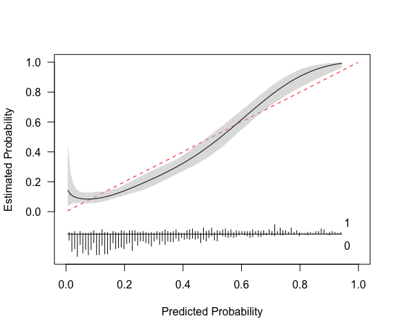
We can use a calibration curve to assess ‘moderate’ calibration.
Below we use pmcalibration to fit a flexible calibration
curve, allowing for a non-linear relationship between predicted and
actual probabilities.
In the example below, we fit a calibration curve using a restricted
cubic spline with 5 knots (see ?rms::rcs).
transf="logit" signals that the predicted risks should be
logit transformed before fitting the calibration curve (this is the
default for a binary y). pmcalibration
calculates various metrics from the absolute difference between the
predicted probability and the actual probability (as estimated by the
calibration curve). In this case 95% confidence intervals for these
metrics are calculated via simulation based inference
(ci = "sim") with 1000 replicates. Alternatively we could
have chosen bootstrap confidence intervals
(ci = "boot").
(cc <- pmcalibration(y = y, p = p,
                     smooth = "rcs", nk = 5,
                     transf="logit",
                     ci = "sim",
                     n=1000))
#> Calibration metrics based on a calibration curve estimated for a binary outcome via a restricted cubic spline (see ?rms::rcs) using logit transformed predicted probabilities.
#>
#>      Estimate lower upper
#> Eavg    0.054 0.035 0.076
#> E50     0.059 0.031 0.079
#> E90     0.083 0.060 0.134
#> Emax    0.138 0.081 0.448
#> ECI     0.368 0.177 0.751
#>
#> 95% confidence intervals calculated via simulation based inference with 1000 replicates.
The printed metrics can be interpreted as follows:
Eavg suggests that the average difference between
prediction and actual probability of the outcome is 0.054 (or 5%) with a
95% CI of [0.035, 0.076].E50 is the median difference between prediction and
observed probability (inferred from calibration curve). 50% of
differences are 0.059 or smaller.E90 is the 90th percentile difference. 90% of
differences are 0.083 or smaller.Emax is the largest observed difference between
predicted and observed probability. The model can be off by up to 0.14,
with a broad confidence interval.ECI is the average squared difference between predicted
and observed probabilities (multiplied by 100). See Van Hoorde et
al. (2015).pmcalibration produces a plot by default, as shown
above. A more custom plot can be obtained via plot.
plot(cc, xlab="Predicted Risk of Outcome", ylab="Expected Proportion with Outcome", fillcol = "blue", ideallty = 0)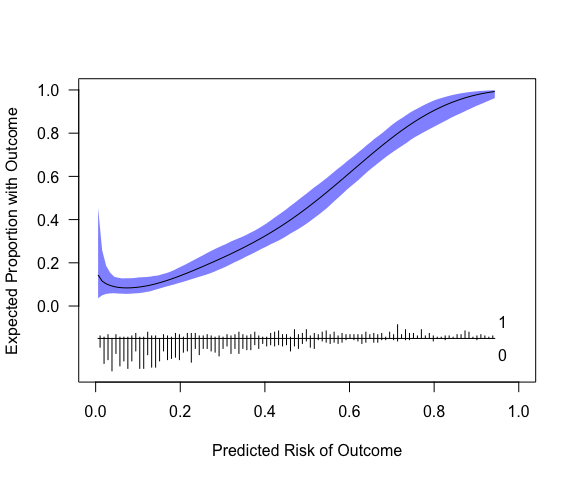
Or one could use get_curve to extract data for plotting
with method of your choice.
pcc <- get_curve(cc)
head(pcc)
#>             p        p_c      lower     upper
#> 1 0.005804309 0.14402182 0.03580601 0.4538340
#> 2 0.015274021 0.11541021 0.04965833 0.2590454
#> 3 0.024743733 0.10296340 0.05610697 0.1868902
#> 4 0.034213445 0.09521032 0.05846271 0.1543373
#> 5 0.043683157 0.08985188 0.05926845 0.1357910
#> 6 0.053152869 0.08642764 0.05780335 0.1307891
# p = predicted risk (x-axis; this is not p provided to pmcalibration but is determined by eval)
# p_c = risk implied by calibration curve (y-axis)
The model in its current form very slightly overestimates risk at low levels of predicted risk and then underestimates risk at predicted probabilities of over around 0.6.
The results above can be compared with rms::val.prob.
Note that this uses lowess(p, y, iter=0) to fit a
calibration curve. In this case lowess results in the curve
extending beyond the possible range of risks, but the Emax, E90, and
Eavg point estimates are consistent with those above.
library(rms)
#> Loading required package: Hmisc
#>
#> Attaching package: 'Hmisc'
#> The following objects are masked from 'package:base':
#>
#>     format.pval, units
val.prob(p = p, y = y) |>
  round(3)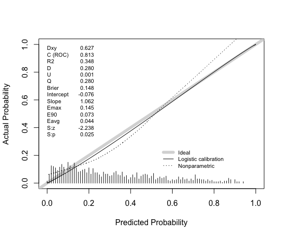
#>       Dxy   C (ROC)        R2         D  D:Chi-sq       D:p         U  U:Chi-sq
#>     0.627     0.813     0.348     0.280   281.217     0.000     0.001     2.566
#>       U:p         Q     Brier Intercept     Slope      Emax       E90      Eavg
#>     0.277     0.280     0.148    -0.076     1.062     0.145     0.073     0.044
#>       S:z       S:p
#>    -2.238     0.025
Note also that the calibration intercept reported by
rms::val.prob comes from the same logistic regression as
that used to estimate the calibration slope. In
logistic_cal the calibration intercept is estimated via a
glm with logit transformed predicted probabilities included
as an offset term (i.e., with slope fixed to 1 - see, e.g., Van Calster et al.,
2016). The calibration slope is estimated via a separate
glm. We can confirm this by accessing the corresponding
estimates from the logistic_cal object.
# access the model used to get calibration slope
# and compare to estimates from val.prob
coef(lcal$calibration_slope) |>
  round(3)
#> (Intercept)          LP
#> -0.076 1.062The code below produces a calibration curve, and associated metrics,
for a time-to-event outcome. The curve has to be constructed for
predictions at a given time point, so an extra argument
time should be specified. Here we use a restricted cubic
spline with 5 knots to assess predictions at time = 15. In this case we
use ci="boot" to get bootstrap confidence intervals for the
metrics and curve (ci="sim" is currently unsupported for
time-to-event outcomes). By default predicted risks are transformed via
the complementary log-log transformation
(function(x) log(-log(1 - x))) before estimating the
calibration curve.
library(simsurv)
library(survival)

# simulate some data
n <- 2000
X <- data.frame(id = seq(n), x1 = rnorm(n), x2 = rnorm(n))
X$x3 <- X$x1*X$x2 # interaction

b <- c("x1" = -.2, "x2" = -.2, "x3" = .1)

d <- simsurv(dist = "weibull", lambdas = .01, gammas = 1.5, x = X, betas = b, seed = 246)

mean(d$eventtime)
#> [1] 19.60637
median(d$eventtime)
#> [1] 16.52855
mean(d$status) # no censoring
#> [1] 1

d <- cbind(d, X[,-1])

head(d)
#>   id eventtime status         x1         x2          x3
#> 1  1 12.749281      1  0.7534077  0.8486379  0.63937033
#> 2  2 24.840161      1  0.4614734 -2.1876625 -1.00954805
#> 3  3  9.087482      1 -0.6338945 -1.8948297  1.20112211
#> 4  4 24.811402      1 -1.0248165  0.6541197 -0.67035271
#> 5  5 19.072266      1 -0.1673414 -0.4625003  0.07739544
#> 6  6 13.595427      1  0.2376988  0.6452848  0.15338343

# split into development and validation
ddev <- d[1:1000, ]
dval <- d[1001:2000, ]

# fit a cox model
cph <- coxph(Surv(eventtime, status) ~ x1 + x2, data = ddev)

# predicted probability of event at time = 15
p = 1 - exp(-predict(cph, type="expected", newdata = data.frame(eventtime=15, status=1, x1=dval$x1, x2=dval$x2)))

y <- with(dval, Surv(eventtime, status))

# calibration curve at time = 15
(cc <- pmcalibration(y = y, p = p, smooth = "rcs", nk = 5,
                     ci = "boot", time = 15))
#> Calibration metrics based on a calibration curve estimated for a time-to-event outcome (time = 15) via a restricted cubic spline (see ?rms::rcs) using complementary log-log transformed predicted probabilities.
#>
#>      Estimate lower upper
#> Eavg    0.051 0.028 0.080
#> E50     0.046 0.020 0.077
#> E90     0.077 0.052 0.126
#> Emax    0.245 0.115 0.407
#> ECI     0.349 0.146 0.813
#>
#> 95% confidence intervals calculated via bootstrap resampling with 1000 replicates.
mtext("time = 15")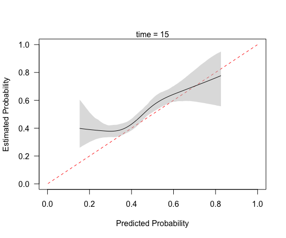
Compare to rms::val.surv, which with the arguments
specified below uses polspline::hare to fit a calibration
curve. Note val.surv uses probability of surviving until
time = u not probability of event occurring by time = u.
(vs <- val.surv(S = y, est.surv = 1-p, u=15,
                fun = function(x) log(-log(x))))
#>
#> Validation of Predicted Survival at Time= 15     n= 1000 , events= 1000
#>
#> hare fit:
#>
#> dim A/D   loglik       AIC        penalty
#>                                 min    max
#>   1 Add  -3949.05   7905.02  148.71     Inf
#>   2 Add  -3874.70   7763.22   60.48  148.71
#>   3 Add  -3844.46   7709.64   32.04   60.48
#>   4 Del  -3828.44   7684.51    7.10   32.04
#>   5 Add  -3824.89   7684.32    0.00    7.10
#>
#> the present optimal number of dimensions is 5.
#> penalty(AIC) was 6.91, the default (BIC), would have been 6.91.
#>
#>   dim1           dim2           beta        SE         Wald
#> Constant                            -2.6       0.25  -10.69
#> Time        26                    -0.031      0.005   -6.27
#> Co-1  linear                       0.063       0.26    0.24
#> Time       7.2                     -0.15      0.028   -5.42
#> Co-1     -0.81                      0.92       0.34    2.74
#>
#> Function used to transform predictions:
#> function (x)  log(-log(x))
#>
#> Mean absolute error in predicted probabilities: 0.0352
#> 0.9 Quantile of absolute errors               : 0.0760
plot(vs, lim=0:1)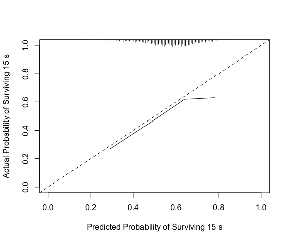
We can make a plot that is easier to compare.
x <- get_curve(cc)

with(x, plot(1-p, 1-p_c, type="l", xlim=0:1, ylim=0:1,
             xlab="Predicted Probability of Surviving 15",
             ylab="Actual Probability of Surviving 15"))
matplot(1-x$p, y = 1-x[, 3:4], type = "l", lty=2,
        col="black", add = TRUE)
abline(0,1, col="red", lty=2)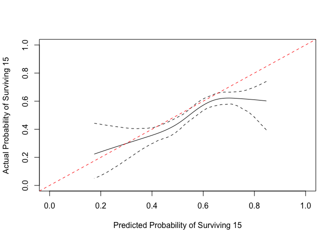
pmcalibration can be used to assess apparent calibration
in a development sample or to externally validate an existing prediction
model. For conducting internal validation (via bootstrap optimism or
cross-validation) users are encouraged to look at https://stephenrho.github.io/pminternal/.