The tvcure package enables to fit additive cure survival model with exogenous time-varying covariates (Lambert & Kreyenfeld, 2025) [1,2].
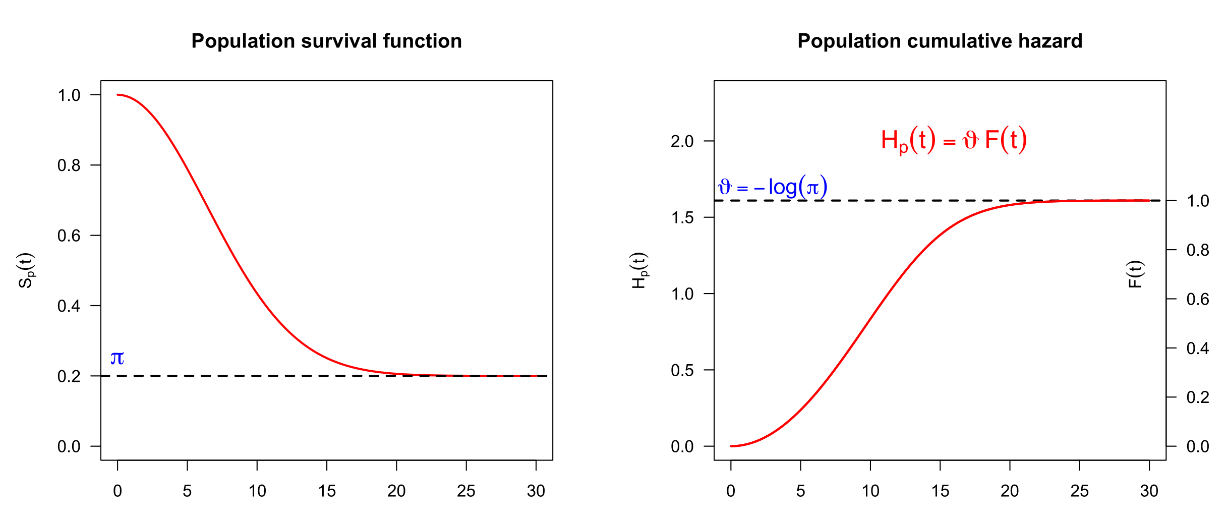
The starting point is the bounded cumulative hazard model (also name the promotion time model) (Tsodikov 1998) with population survival function \[S_p(t|\mathbf{v}) = \exp\{-H_p(t|\mathbf{v})\} =\exp\{-{\vartheta(\mathbf{v})} F(t)\},\] bounded hazard \(H_p(t|\mathbf{v})\) and cure fraction \(\pi(\mathbf{v})=S_p(+\infty|\mathbf{v})=\exp\{-{\vartheta(\mathbf{v})}\}\), see Figure 1. Function \(F(t)\) is a c.d.f. governing the population hazard dynamics, with \(F(0)=1\) and \(F(T)=1\) where \(T\) is the minimum value of time after which an event-free unit is considered cured.
The extended promotion model (Bremhorst and Lambert 2016) additionally allows the event dynamics governed by \(F(t)\) to change with covariates \(\tilde{\mathbf{v}}\), \[S_p(t|\mathbf{v},\tilde{\mathbf{v}}) = \exp\{-H_p(t|\mathbf{v},\tilde{\mathbf{v}})\} =\exp\{-{\vartheta(\mathbf{v})} {F(t|\tilde{\mathbf{v}})}\}\]
For categorical covariates \({\mathbf z}\) and continuous covariates \({\mathbf x}\), the following additive long-term survival submodel defining the cure probability is assumed, \(\vartheta(\mathbf{v})= -\log \pi(\mathbf{v}) =\exp\{\eta_\vartheta(\mathbf{v})\}\) where \(\eta_\vartheta(\mathbf{v}) = \beta_0 + {\pmb \beta}^\top{\mathbf z} + \sum_j f_j(x_j)\), a positive value for \(\beta_k\) suggesting an event probability increasing with \(z_k\) and, consequently, a cure probability decreasing with \(z_k\). The event dynamics is governed by the additive short-term submodel, \(F(t|\tilde{\mathbf{v}}) = 1-S_0(t)^{\exp(\eta_F(\tilde{\mathbf{v}}))}\), where \(\eta_F(\tilde{\mathbf{v}})= {\pmb{\gamma}}^\top\tilde{\mathbf{z}} + \sum_j \tilde{f}_j(\tilde{x}_j)\), a positive value for \(\gamma_k\) suggesting an acceleration of event timing with \(z_k\), see Bremhorst, Kreyenfeld & Lambert (2019). The baseline density function \(f_0(t)=-{d\over dt}S_0(t)\) and the additive terms are specified using Bayesian P-splines. The model is identifiable provided that the follow-up is sufficiently long to display the plateau in the population survival function (Lambert & Bremhorst, 2019).
The core contribution in Lambert and Kreyenfeld (2025) is an extension of that model to include exogenous time-varying covariates. The model specification starts with the population hazard function from which other quantities can be obtained: \[h_p(t|\mathbf{v}(t),\tilde{\mathbf{v}}(t)) = \vartheta(\mathbf{v}(t)) f(t|\tilde{\mathbf{v}}(t)) = \mathrm{e}^{\eta_\vartheta(\mathbf{v}(t))+\eta_F(\tilde{\mathbf{v}}(t))} f_0(t)S_0(t)^{\exp(\eta_F(\tilde{\mathbf{v}}(t))-1}\] In the special case where covariates are constant, we return to the preceding extended promotion time model with static covariates.
The combination of Laplace approximations and of Bayesian P-splines (named LPS) enable fast and flexible inference in a Bayesian framework (Lambert & Gressani, 2023). The Gaussian Markov field prior assumed for the penalized spline parameters and the Bernstein-von Mises theorem provide reliable Laplace approximation to the posterior distribution of these quantities.
Let us illustrate the use of the tvcure package on simulated right-censored data:
## Package installation and loading
## install.packages("devtools")
## devtools::install_github("plambertULiege/tvcure")
library(tvcure)

## Data simulation
beta = c(beta0=.4, beta1=-.2, beta2=.15) ; gam = c(gam1=.2, gam2=.2)
data = simulateTVcureData(n=500, seed=123, beta=beta, gam=gam,
                        RC.dist="exponential",mu.cens=550)$rawdata
round(head(data),3)
## id time event z1 z2 x1 x2 z3 z4 x3 x4
## 1 1 1 0 0.5 -0.086 0.945 0.199 0.5 -0.053 0.945 0.184
## 2 1 2 0 0.5 -0.086 0.932 0.198 0.5 -0.053 0.932 0.202
## 3 1 3 0 0.5 -0.086 0.918 0.196 0.5 -0.053 0.918 0.219
## 4 1 4 0 0.5 -0.086 0.905 0.195 0.5 -0.053 0.905 0.236
## 5 1 5 0 0.5 -0.086 0.891 0.193 0.5 -0.053 0.891 0.252
## 6 1 6 0 0.5 -0.086 0.878 0.192 0.5 -0.053 0.878 0.269The data frame should always have a counting process form and contain at least the following entries:
id: the id of the unit associated to the data in a given line in the data frame.
time: the integer time at which the observations are reported. For a given unit, it should be a sequence of consecutive integers starting at 1 for the first observation.
event : a sequence of 0-1 event indicators. For the lines corresponding to a given unit, it starts with 0 values concluded by a 0 in case of right-censoring or by a 1 if the event is observed at the end of the follow-up.
Let us fit a double additive tvcure model to these data with:
categorical covariates \(z_1, z_2\) and continous covariates \(x_1\) and \(x_2\) entering in an additive way in the long-term survival submodel ;
categorical covariates \(z_3, z_4\) and continous covariates \(x_3\) and \(x_4\) entering in an additive way in the short-term survival submodel.
model = tvcure(~z1+z2+s(x1)+s(x2),
               ~z3+z4+s(x3)+s(x4), data=data)
print(model)
##
## Call:
## tvcure(formula1 = ~z1 + z2 + s(x1) + s(x2), formula2 = ~z3 +
## z4 + s(x3) + s(x4), data = data)
##
## Prior on penalty parameter(s): Gamma(1,1e-04)
##
## >> log(theta(x)) - Long-term survival (Quantum) <<
## Formula: ~z1 + z2 + s(x1) + s(x2)
##
## Parametric coefficients:
## est se low up Z Pval
## (Intercept) 0.493 0.067 0.362 0.625 7.35 <0.001 ***
## z1 -0.109 0.107 -0.319 0.101 -1.02 0.308
## z2 0.212 0.055 0.105 0.319 3.87 <0.001 ***
##
## exp(est) exp(-est) low up Pval
## z1 0.897 1.115 0.727 1.106 0.308
## z2 1.236 0.809 1.110 1.376 <0.001 ***
##
## Approximate significance of smooth terms (Wood's <Tr> or Chi2):
## edf Tr Pval Chi2 Pval
## f1(x1) 1.63 8.43 0.01 8.60 0.009 **
## f1(x2) 3.18 24.46 <0.001 28.65 <0.001 ***
##
## >> eta(x) - Short-term survival (Timing) <<
## Formula: ~z3 + z4 + s(x3) + s(x4)
##
## Parametric coefficients:
## est se low up Z Pval
## z3 0.216 0.138 -0.053 0.486 1.57 0.116
## z4 0.185 0.070 0.048 0.322 2.64 0.008 **
##
## exp(est) exp(-est) low up Pval
## z3 1.241 0.806 0.948 1.626 0.116
## z4 1.203 0.831 1.049 1.380 0.008 **
##
## Approximate significance of smooth terms (Wood's <Tr> or Chi2):
## edf Tr Pval Chi2 Pval
## f2(x3) 2.55 9.16 0.021 9.64 0.015 *
## f2(x4) 1.19 3.04 0.112 2.91 0.112
##
## ---------------------------------------------------------------
## logEvid: -2018.52 Dev: 3163.45 AIC: 3190.56 BIC: 3242.98
## edf: 13.56 nobs: 50672 n: 500 (units) d: 353 (events)
## Convergence: TRUE -- Algorithms: NR-LPS / LM-LPS
## Elapsed time: 6.1 seconds (16 iterations)
## ---------------------------------------------------------------The estimated reference hazard \(\mathrm{e}^{\beta_0}f_0(t)\) and the associated c.d.f. function \(F_0(t)\) governing the baseline dynamics of the cumulative hazard can also visualized,
plot(model, select=0, pages=1)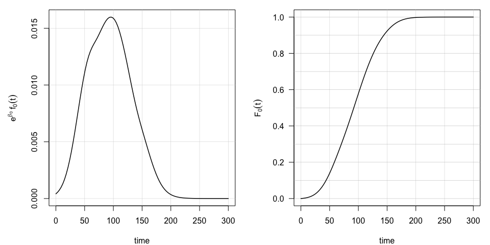 as well as the estimated additive terms in the long-term survival
submodel,
as well as the estimated additive terms in the long-term survival
submodel,
plot(model, select=c(1,2), pages=1) ## First 2 additive terms in the model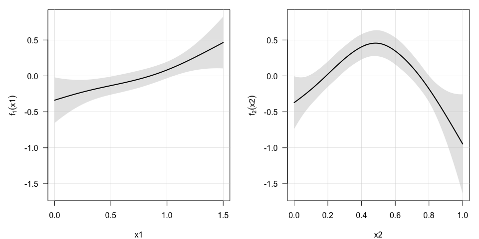 or in the short-term survival submodel,
plot(model, select=c(3,4), pages=1) ## Last 2 additive terms in the model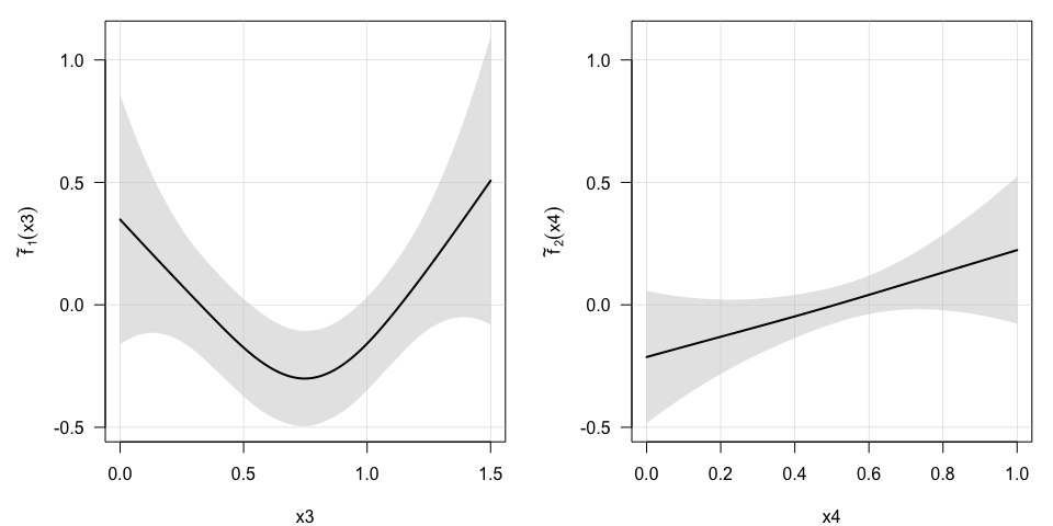
It is possible to force the additive terms to be zero for selected reference values for the covariates, which facilitates the interpretation of the other model parameters:
model = tvcure(~z1+z2+s(x1,ref=.75)+s(x2,ref=.5),
               ~z3+z4+s(x3,ref=.75)+s(x4,ref=.5), data=data)
plot(model, select=1:4, pages=1) ## The 4 additive terms in the model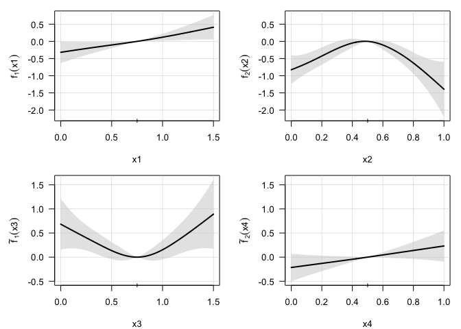
Predictions can be made for a given history of covariate values. Consider for example unit 1 for which no event was observed by the end of the follow-up:
data1 = subset(data, data$id==1) ## Data for unit 1
round(tail(data1, n=1),3) ## Data at the last observation time
## id time event z1 z2 x1 x2 z3 z4 x3 x4
## 275 1 275 0 -0.5 -0.086 0.668 0.104 -0.5 -0.053 0.668 0.336The estimated population survival function of a subject sharing the same covariate history can be computed and visualized,
obj = predict(model, ci.level=0.95, newdata=data1)
matplot(obj$Sp, ylim=c(0,1),
        type="l", lty=c(1,2,2), col=1, las=1,
        xlab="time", ylab=bquote(S[p](t)))
grid(lwd=.5,lty=1)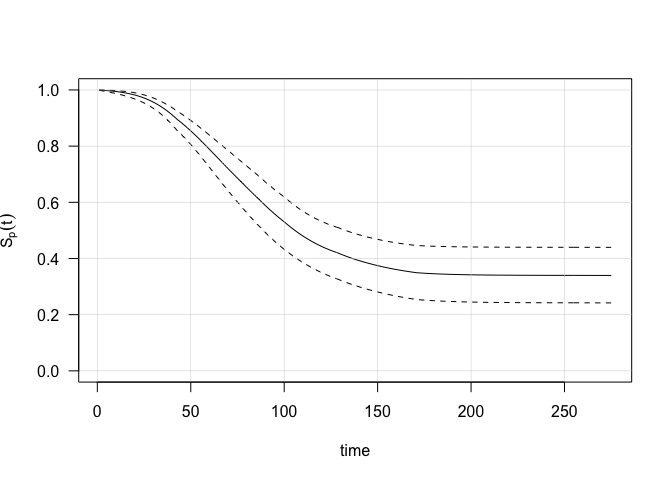
with the last value providing the estimated cure probability (with credible bounds):
print(tail(obj$Sp,n=1)) ## Cure probability## est low up
## [275,] 0.3396353 0.241924 0.4396692More details can be found in Lambert & Kreyenfeld (2025) and in the documentation of the tvcure package.
tvcure: Additive cure survival model with exogenous time-varying covariates. Copyright (C) 2023-2025 Philippe Lambert
This program is free software: you can redistribute it and/or modify it under the terms of the GNU General Public License as published by the Free Software Foundation, either version 3 of the License, or (at your option) any later version.
This program is distributed in the hope that it will be useful, but WITHOUT ANY WARRANTY; without even the implied warranty of MERCHANTABILITY or FITNESS FOR A PARTICULAR PURPOSE. See the GNU General Public License for more details.
You should have received a copy of the GNU General Public License along with this program. If not, see https://www.gnu.org/licenses/.
[1] Lambert, P. and Kreyenfeld, M. (2025). Time-varying exogenous covariates with frequently changing values in double additive cure survival model: an application to fertility. Journal of the Royal Statistical Society, Series A. doi:10.1093/jrsssa/qnaf035
[2] Lambert, P. (2025). R-package tvcure - Version 0.6.6. GitHub: plambertULiege/tvcure
[3] Lambert, P. and Gressani, O. (2023). Penalty parameter selection and asymmetry corrections to Laplace approximations in Bayesian P-splines models. Statistical Modelling, 23(5-6): 409–423. doi:10.1177/1471082X231181173
[4] Lambert, P. and Bremhorst, V. (2020). Inclusion of time-varying covariates in cure survival models with an application in fertility studies. Journal of the Royal Statistical Society, Series A, 183(1): 333-354. doi:10.1111/rssa.12501
[5] Lambert, P. and Bremhorst, V. (2019). Estimation and identification issues in the promotion time cure model when the same covariates influence long- and short-term survival. Biometrical Journal, 61(2): 275-279. doi:10.1002/bimj.201700250
[6] Gressani, O. and Lambert P. (2018). Fast Bayesian inference using Laplace approximations in a flexible promotion time cure model based on P-splines. Computational Statistics and Data Analysis, 124: 151-167. doi:10.1016/j.csda.2018.02.007
[7] Bremhorst, V., Kreyenfeld M. and Lambert P. (2019). Nonparametric double additive cure survival models: an application to the estimation of the nonlinear effect of age at first parenthood on fertility progression. Statistical Modelling, 19(3): 248-275. doi:10.1177/1471082X18784685
[8] Bremhorst, V., Kreyenfeld M. and Lambert P. (2016). Fertility progression in Germany: an analysis using flexible nonparametric cure survival models. Demographic Research, 35: 505-534. doi:10.4054/DemRes.2016.35.18
[9] Bremhorst, V. and Lambert, P. (2016). Flexible estimation in cure survival models using Bayesian P-splines. Computational Statistics and Data Analysis, 93, 270–284. doi:10.1016/j.csda.2014.05.009
[10] Tsodikov, A. (1998) A proportional hazard model taking account of long-term survivors. Biometrics, 54, 1508–1516. doi:10.2307/2533675