Title:	Utility Functions to Support and Extend the 'rbmi' Package
Version:	0.3.0
Date:	2026-02-14
Maintainer:	Mark Baillie <bailliem@gmail.com>
Description:	Provides utility functions that extend the capabilities of the reference-based multiple imputation package 'rbmi'. It supports clinical trial analysis workflows with functions for managing imputed datasets, applying analysis methods across imputations, and tidying results for reporting.
License:	GPL (≥ 3)
Encoding:	UTF-8
RoxygenNote:	7.3.2
Suggests:	cards, ggplot2, gt, knitr, patchwork, readr, rmarkdown, rstan, spelling, testthat (≥ 3.0.0), tibble
Config/testthat/edition:	3
Language:	en-US
Imports:	assertthat, beeca, cli (≥ 3.6.0), dplyr, lifecycle (≥ 1.0.4), purrr, rbmi (≥ 1.4), rlang, tidyr
VignetteBuilder:	knitr
Depends:	R (≥ 4.1)
LazyData:	true
URL:	https://github.com/openpharma/rbmiUtils
BugReports:	https://github.com/openpharma/rbmiUtils/issues
NeedsCompilation:	no
Packaged:	2026-02-16 21:09:40 UTC; bailliem
Author:	Mark Baillie [aut, cre, cph], Tobias Muetze [aut], Jack Talboys [aut], Lukas A. Widmer [ctb]
Repository:	CRAN
Date/Publication:	2026-02-16 21:40:02 UTC

rbmiUtils: Utility Functions to Support and Extend the 'rbmi' Package

Description

Provides utility functions that extend the capabilities of the reference-based multiple imputation package 'rbmi'. It supports clinical trial analysis workflows with functions for managing imputed datasets, applying analysis methods across imputations, and tidying results for reporting.

Author(s)

Maintainer: Mark Baillie bailliem@gmail.com (ORCID) [copyright holder]

Authors:

• Tobias Muetze tobias.muetze@novartis.com (ORCID)

• Jack Talboys jack.talboys@novartis.com

Other contributors:

• Lukas A. Widmer (ORCID) [contributor]

See Also

Useful links:

• https://github.com/openpharma/rbmiUtils

• Report bugs at https://github.com/openpharma/rbmiUtils/issues

Example efficacy trial dataset

Description

A simplified example of a simulated trial dataset, with missing data.

Usage

ADEFF

Format

ADEFF A data frame with 1,000 rows and 10 columns:

USUBJID

Unique subject identifier

AVAL

Primary outcome variable

TRT01P

Planned treatment

STRATA

Stratification at randomisation

REGION

Stratification by region

REGIONC

Stratification by region, numeric code

BASE

Baseline value of primary outcome variable

CHG

Change from baseline

AVISIT

Visit number

PARAM

Analysis parameter name

Example multiple imputation trial dataset

Description

A simplified example of a simulated trial ADMI dataset

Usage

ADMI

Format

ADMI A data frame with 100,000 rows and 12 columns:

USUBJID

Unique patient identifier

STRATA

Stratification at randomisation

REGION

Stratification by region

REGIONC

Stratification by region, numeric code

TRT

Planned treatment

BASE

Baseline value of primary outcome variable

CHG

Change from baseline

AVISIT

Visit number

IMPID

Imputation number identifier

CRIT1FLN

Responder criteria (binary)

CRIT1FL

Responder criteria (categorical)

CRIT

Responder criteria (definition)

Apply Analysis Function to Multiple Imputed Datasets

Description

This function applies an analysis function (e.g., ANCOVA) to imputed datasets and stores the results for later pooling. It is designed to work with multiple imputed datasets and apply a given analysis function to each imputation iteration.

Usage

analyse_mi_data(
  data = NULL,
  vars = NULL,
  method = NULL,
  fun = rbmi::ancova,
  delta = NULL,
  ...
)

Arguments

Details

The function loops through distinct imputation datasets (identified by IMPID), applies the provided analysis function fun, and stores the results for later pooling. If a delta dataset is provided, it will be merged with the imputed data to apply the specified delta adjustment before analysis.

Workflow:

1. Prepare imputed data using get_imputed_data() or expand_imputed_data()

2. Define variables using rbmi::set_vars()

3. Call analyse_mi_data() to apply analysis to each imputation

4. Pool results using rbmi::pool()

5. Tidy results using tidy_pool_obj()

Value

An object of class analysis containing the results from applying the analysis function to each imputed dataset. Pass this to rbmi::pool() to obtain pooled estimates.

See Also

• rbmi::analyse() which this function wraps

• rbmi::pool() for pooling the analysis results

• The rbmi quickstart vignette

• tidy_pool_obj() to format pooled results for publication

• get_imputed_data() to extract imputed datasets from rbmi objects

• expand_imputed_data() to reconstruct full imputed data from reduced form

• gcomp_responder_multi() for binary outcome analysis

• validate_data() to check data before imputation

Examples

# Example usage with an ANCOVA function
library(dplyr)
library(rbmi)
library(rbmiUtils)
set.seed(123)
data("ADMI")

# Convert key columns to factors
ADMI$TRT <- factor(ADMI$TRT, levels = c("Placebo", "Drug A"))
ADMI$USUBJID <- factor(ADMI$USUBJID)
ADMI$AVISIT <- factor(ADMI$AVISIT)

# Define key variables for ANCOVA analysis
 vars <- set_vars(
  subjid = "USUBJID",
  visit = "AVISIT",
  group = "TRT",
  outcome = "CHG",
  covariates = c("BASE", "STRATA", "REGION")  # Covariates for adjustment
 )

# Specify the imputation method (Bayesian) - need for pool step
 method <- rbmi::method_bayes(
 n_samples = 20,
 control = rbmi::control_bayes(
   warmup = 20,
   thin = 1
   )
 )

# Perform ANCOVA Analysis on Each Imputed Dataset
ana_obj_ancova <- analyse_mi_data(
  data = ADMI,
  vars = vars,
  method = method,
  fun = ancova,  # Apply ANCOVA
  delta = NULL   # No sensitivity analysis adjustment
)

Construct an rbmi analysis object

Description

This is a helper function to create an analysis object that stores the results from multiple imputation analyses. It validates the results and ensures proper class assignment.

This is a modification of the rbmi::as_analysis function. This function is deprecated and will be removed in a future version.

Usage

as_analysis2(results, method, delta = NULL, fun = NULL, fun_name = NULL)

Arguments

Value

An object of class analysis with the results and associated metadata.

Convert character variable list to formula

Description

This function is deprecated and will be removed in a future version.

Usage

as_simple_formula2(outcome, covars)

Arguments

Value

A formula object.

Combine Results Across Multiple Analyses

Description

Combines tidy result tibbles from multiple analyses (e.g., different endpoints or subgroups) into a single table with an identifying column.

Usage

combine_results(..., results_list = NULL, id_col = "analysis")

Arguments

Value

A tibble with all results combined, with an additional column identifying the source analysis.

See Also

• tidy_pool_obj() to create tidy results from pooled objects

• format_results() to format combined results for reporting

Examples

library(rbmi)
library(dplyr)

# Assuming you have multiple pooled results
# results_week24 <- tidy_pool_obj(pool_obj_week24)
# results_week48 <- tidy_pool_obj(pool_obj_week48)

# Combine them
# combined <- combine_results(
#   "Week 24" = results_week24,
#   "Week 48" = results_week48
# )

Create IMPID Column for Imputed Datasets

Description

Adds an IMPID column to a list of imputed datasets, converting them to a single stacked data.frame suitable for use with analyse_mi_data().

Usage

create_impid(imputed_list, id_prefix = "")

Arguments

Details

This function is useful when you have imputed datasets from a source other than rbmi (e.g., from mice or another MI package) and want to use them with rbmiUtils analysis functions.

Value

A single data.frame with all imputed datasets stacked, with an IMPID column identifying the source imputation.

See Also

• get_imputed_data() to extract imputed data from rbmi objects

• analyse_mi_data() to analyse stacked imputed data

Examples

# Create example imputed datasets
imp1 <- data.frame(USUBJID = c("S1", "S2"), CHG = c(1.5, 2.5))
imp2 <- data.frame(USUBJID = c("S1", "S2"), CHG = c(1.8, 2.2))
imp3 <- data.frame(USUBJID = c("S1", "S2"), CHG = c(1.6, 2.4))

# Stack with IMPID
stacked <- create_impid(list(imp1, imp2, imp3))
print(stacked)

Describe an rbmi Draws Object

Description

Extracts structured metadata from an rbmi draws object, including method, formula, sample count, failures, covariance structure, and (for Bayesian methods) MCMC convergence diagnostics. Returns an S3 object with an informative print() method.

Usage

describe_draws(draws_obj)

Arguments

Details

For conditional mean methods, the sample count is displayed as "1 + N" matching the rbmi convention where the first sample is the primary (full-data) fit and the remaining N are jackknife or bootstrap resamples.

For Bayesian methods, MCMC convergence diagnostics (ESS, Rhat) are extracted from the stanfit object when rstan is available. The converged flag uses the Rhat < 1.1 threshold matching rbmi's own convention.

Value

An S3 object of class c("describe_draws", "list") containing:

method

Human-readable method name (e.g., "Bayesian (MCMC via Stan)")

method_class

Raw class name: "bayes", "approxbayes", or "condmean"

n_samples

Total number of samples

n_failures

Number of failed samples

formula

Deparsed model formula string

covariance

Covariance structure (e.g., "us")

same_cov

Logical; whether same covariance is used across groups

condmean_type

(condmean only) "jackknife" or "bootstrap"

n_primary

(condmean only) Always 1

n_resampled

(condmean only) Number of resampled draws

bayes_control

(bayes only) List with warmup, thin, chains, seed

mcmc

(bayes with stanfit only) List with rhat, ess, max_rhat, min_ess, n_params, converged

See Also

• rbmi::draws() to create draws objects

• rbmi::method_condmean(), rbmi::method_bayes(), rbmi::method_approxbayes() for method specification

Examples

## Not run: 
library(rbmi)
library(dplyr)
data("ADEFF", package = "rbmiUtils")

# Prepare ADEFF data for rbmi pipeline
ADEFF <- ADEFF |>
  mutate(
    TRT = factor(TRT01P, levels = c("Placebo", "Drug A")),
    USUBJID = factor(USUBJID),
    AVISIT = factor(AVISIT, levels = c("Week 24", "Week 48"))
  )

vars <- set_vars(
  subjid = "USUBJID", visit = "AVISIT", group = "TRT",
  outcome = "CHG", covariates = c("BASE", "STRATA", "REGION")
)
dat <- ADEFF |> select(USUBJID, STRATA, REGION, TRT, BASE, CHG, AVISIT)
draws_obj <- draws(
  data = dat, vars = vars,
  method = method_bayes(n_samples = 100)
)

# Inspect the draws object
desc <- describe_draws(draws_obj)
print(desc)

# Programmatic access to metadata
desc$method
desc$n_samples
desc$formula

## End(Not run)

Describe an rbmi Imputation Object

Description

Extracts structured metadata from an rbmi imputation object, including method, number of imputations (M), reference arm mappings, subject count, and a missingness breakdown by visit and treatment arm. Returns an S3 object with an informative print() method.

Usage

describe_imputation(impute_obj)

Arguments

Details

The missingness table is built by cross-tabulating impute_obj$data$is_missing by visit and treatment group. Each row shows the total number of subjects in that group, how many had missing data at that visit, and the percentage missing.

Value

An S3 object of class c("describe_imputation", "list") containing:

method

Human-readable method name (e.g., "Bayesian (MCMC via Stan)")

method_class

Raw class name: "bayes", "approxbayes", or "condmean"

n_imputations

Number of imputations (M)

references

Named character vector of reference arm mappings, or NULL

n_subjects

Total number of unique subjects

visits

Character vector of visit names

missingness

A data.frame with columns: visit, group, n_total, n_miss, pct_miss

See Also

• rbmi::impute() to create imputation objects

• describe_draws() for inspecting draws objects

Examples

## Not run: 
library(rbmi)
library(dplyr)
data("ADEFF", package = "rbmiUtils")

ADEFF <- ADEFF |>
  mutate(
    TRT = factor(TRT01P, levels = c("Placebo", "Drug A")),
    USUBJID = factor(USUBJID),
    AVISIT = factor(AVISIT, levels = c("Week 24", "Week 48"))
  )

vars <- set_vars(
  subjid = "USUBJID", visit = "AVISIT", group = "TRT",
  outcome = "CHG", covariates = c("BASE", "STRATA", "REGION")
)
dat <- ADEFF |> select(USUBJID, STRATA, REGION, TRT, BASE, CHG, AVISIT)
draws_obj <- draws(
  data = dat, vars = vars,
  method = method_bayes(n_samples = 100)
)
impute_obj <- impute(
  draws_obj,
  references = c("Placebo" = "Placebo", "Drug A" = "Placebo")
)

# Inspect the imputation
desc <- describe_imputation(impute_obj)
print(desc)

# Programmatic access
desc$n_imputations
desc$missingness
desc$references

## End(Not run)

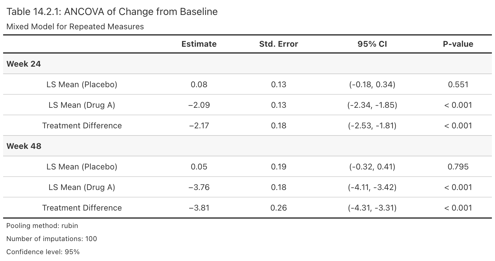
Create Regulatory-Style Efficacy Summary Table

Description

Takes an rbmi pool object and produces a publication-ready gt table in the style of CDISC/ICH Table 14.2.x. The table displays least squares means by treatment arm, treatment differences, confidence intervals, and p-values, organized by visit row groups.

Usage

efficacy_table(
  pool_obj,
  title = NULL,
  subtitle = NULL,
  digits = 2,
  ci_level = NULL,
  arm_labels = NULL,
  pval_digits = 3,
  pval_threshold = 0.001,
  font_family = NULL,
  font_size = NULL,
  row_padding = NULL,
  ...
)

Arguments

Details

This function assumes a single-parameter-per-visit pool object (the standard output from an rbmi ANCOVA or MMRM pipeline). It internally calls tidy_pool_obj() to parse the pool object, then constructs the gt table.

Arm labels: Use the arm_labels parameter to customize arm names in the table. For example, arm_labels = c(ref = "Placebo", alt = "Drug A") will display "LS Mean (Placebo)" and "LS Mean (Drug A)" instead of the defaults.

Customization: The returned gt object can be further customized using standard gt piping, e.g., efficacy_table(pool_obj) |> gt::tab_options(...).

Example output:

Value

A gt table object of class gt_tbl.

See Also

• tidy_pool_obj() for the underlying data transformation

• format_pvalue() for p-value formatting rules

• rbmi::pool() to create pool objects

Examples

if (requireNamespace("gt", quietly = TRUE)) {
  library(rbmi)
  data("ADMI", package = "rbmiUtils")
  ADMI$TRT <- factor(ADMI$TRT, levels = c("Placebo", "Drug A"))
  ADMI$USUBJID <- factor(ADMI$USUBJID)
  ADMI$AVISIT <- factor(ADMI$AVISIT)

  vars <- set_vars(
    subjid = "USUBJID", visit = "AVISIT", group = "TRT",
    outcome = "CHG", covariates = c("BASE", "STRATA", "REGION")
  )
  method <- method_bayes(
    n_samples = 20,
    control = control_bayes(warmup = 20, thin = 1)
  )

  ana_obj <- analyse_mi_data(ADMI, vars, method, fun = ancova)
  pool_obj <- pool(ana_obj)

  # Basic table
  tbl <- efficacy_table(pool_obj)

  # Publication-styled table
  efficacy_table(
    pool_obj,
    title = "Table 14.2.1: ANCOVA of Change from Baseline",
    subtitle = "Mixed Model for Repeated Measures",
    arm_labels = c(ref = "Placebo", alt = "Drug A"),
    font_size = 12,
    row_padding = 4
  )
}

Expand Reduced Imputed Data to Full Dataset

Description

Reconstructs the full imputed dataset from a reduced form by merging imputed values back with the original observed data. This is the inverse operation of reduce_imputed_data().

Usage

expand_imputed_data(reduced_data, original_data, vars)

Arguments

Details

For each imputation (identified by IMPID), this function:

1. Starts with the original data (observed values)

2. Replaces missing outcome values with the corresponding imputed values

3. Stacks all imputations together

Value

A data.frame containing the full imputed dataset with one complete dataset per IMPID value. The structure matches the output of get_imputed_data().

See Also

• rbmi::impute() which creates the imputed datasets this function operates on

• reduce_imputed_data() to create the reduced dataset

• get_imputed_data() to extract imputed data from an rbmi imputation object

Examples

library(rbmi)
library(dplyr)

# Example with package data
data("ADMI", package = "rbmiUtils")
data("ADEFF", package = "rbmiUtils")

# Prepare original data to match ADMI structure
original <- ADEFF |>
  mutate(
    TRT = TRT01P,
    USUBJID = as.character(USUBJID)
  )

vars <- set_vars(
  subjid = "USUBJID",
  visit = "AVISIT",
  group = "TRT",
  outcome = "CHG"
)

# Reduce and then expand
reduced <- reduce_imputed_data(ADMI, original, vars)
expanded <- expand_imputed_data(reduced, original, vars)

# Verify expansion
cat("Original ADMI rows:", nrow(ADMI), "\n")
cat("Expanded rows:", nrow(expanded), "\n")

Extract variable names from model terms

Description

Takes a character vector including potentially model terms like * and : and extracts out the individual variables. This function is deprecated and will be removed in a future version.

Usage

extract_covariates2(x)

Arguments

Value

A character vector of unique variable names.

Extract Least Squares Means

Description

Convenience function to extract only least squares mean estimates from tidy results.

Usage

extract_lsm(results, visit = NULL, arm = NULL)

Arguments

Value

A tibble containing only LSM rows.

See Also

• tidy_pool_obj() to create tidy results

• extract_trt_effects() to extract treatment effects

Examples

library(rbmi)

# Assuming you have a tidy result
# tidy_result <- tidy_pool_obj(pool_obj)
# all_lsm <- extract_lsm(tidy_result)
# ref_lsm <- extract_lsm(tidy_result, arm = "ref")

Extract Treatment Effect Estimates

Description

Convenience function to extract only treatment comparison estimates from tidy results, filtering out least squares means.

Usage

extract_trt_effects(results, visit = NULL)

Arguments

Value

A tibble containing only treatment effect rows.

See Also

• tidy_pool_obj() to create tidy results

• extract_lsm() to extract least squares means

Examples

library(rbmi)

# Assuming you have a tidy result
# tidy_result <- tidy_pool_obj(pool_obj)
# trt_effects <- extract_trt_effects(tidy_result)
# trt_week24 <- extract_trt_effects(tidy_result, visit = "Week 24")

Format Estimate with Confidence Interval

Description

Formats a point estimate with its confidence interval in standard publication format: "estimate (lower, upper)".

Usage

format_estimate(estimate, lower, upper, digits = 2, sep = ", ")

Arguments

Details

The function formats estimates as "X.XX (X.XX, X.XX)" by default. All three input vectors must have the same length. NA values in any position result in NA_character_ for that element.

Value

A character vector of formatted estimates with confidence intervals.

Examples

# Single estimate
format_estimate(1.5, 0.8, 2.2)
#> "1.50 (0.80, 2.20)"

# Multiple estimates
format_estimate(
  estimate = c(-2.5, -1.8),
  lower = c(-4.0, -3.2),
  upper = c(-1.0, -0.4)
)
#> "-2.50 (-4.00, -1.00)" "-1.80 (-3.20, -0.40)"

# More decimal places
format_estimate(0.234, 0.123, 0.345, digits = 3)
#> "0.234 (0.123, 0.345)"

# Different separator
format_estimate(1.5, 0.8, 2.2, sep = " to ")
#> "1.50 (0.80 to 2.20)"

Format P-values for Publication

Description

Formats p-values according to common publication standards, with configurable thresholds and decimal places.

Usage

format_pvalue(x, digits = 3, threshold = 0.001, html = FALSE)

Arguments

Details

The function applies the following rules:

• P-values below threshold are formatted as "< 0.001" (or HTML equivalent)

• P-values >= threshold are rounded to digits decimal places

• NA values are preserved as NA_character_

• Values > 1 or < 0 return NA_character_ with a warning

Value

A character vector of formatted p-values.

Examples

# Basic usage
format_pvalue(0.0234)
#> "0.023"

format_pvalue(0.00005)
#> "< 0.001"

# Vector input
pvals <- c(0.5, 0.05, 0.001, 0.0001, NA)
format_pvalue(pvals)
#> "0.500" "0.050" "0.001" "< 0.001" NA

# Custom threshold
format_pvalue(0.005, threshold = 0.01)
#> "< 0.01"

# HTML output
format_pvalue(0.0001, html = TRUE)
#> "&lt; 0.001"

Format Results for Reporting

Description

Formats a tidy results tibble for publication-ready reporting, with options for rounding, confidence interval formatting, and column selection.

Usage

format_results(
  results,
  digits = 2,
  ci_format = c("parens", "brackets", "dash"),
  pval_digits = 3,
  include_se = FALSE
)

Arguments

Value

A tibble with formatted columns suitable for reporting.

See Also

• tidy_pool_obj() to create tidy results

• combine_results() to combine multiple analyses

Examples

library(rbmi)

# Assuming you have a tidy result
# tidy_result <- tidy_pool_obj(pool_obj)
# formatted <- format_results(tidy_result, digits = 3, ci_format = "brackets")

Format Results Table for Publication

Description

Adds formatted columns to a tidy results table, creating publication-ready output with properly formatted estimates, confidence intervals, and p-values.

Usage

format_results_table(
  data,
  est_col = "est",
  lci_col = "lci",
  uci_col = "uci",
  pval_col = "pval",
  est_digits = 2,
  pval_digits = 3,
  pval_threshold = 0.001,
  ci_sep = ", "
)

Arguments

Details

This function is designed to work with output from tidy_pool_obj() but can be used with any data.frame containing estimate, CI, and p-value columns. The original columns are preserved; new formatted columns are added.

Value

A tibble with additional formatted columns:

est_ci

Formatted estimate with confidence interval

pval_fmt

Formatted p-value

Examples

library(dplyr)

# Create example results
results <- tibble::tibble(
  parameter = c("trt_Week24", "lsm_ref_Week24", "lsm_alt_Week24"),
  description = c("Treatment Effect", "LS Mean (Reference)", "LS Mean (Treatment)"),
  est = c(-2.45, 5.20, 2.75),
  se = c(0.89, 0.65, 0.71),
  lci = c(-4.20, 3.93, 1.36),
  uci = c(-0.70, 6.47, 4.14),
  pval = c(0.006, NA, NA)
)

# Format for publication
formatted <- format_results_table(results)
print(formatted[, c("description", "est_ci", "pval_fmt")])

Utility function for Generalized G-computation for Binary Outcomes

Description

Wrapper function for targeting a marginal treatment effect using g-computation using the beeca package. Intended for binary endpoints.

Usage

gcomp_binary(
  data,
  outcome = "CRIT1FLN",
  treatment = "TRT",
  covariates = c("BASE", "STRATA", "REGION"),
  reference = "Placebo",
  contrast = "diff",
  method = "Ge",
  type = "HC0",
  ...
)

Arguments

Value

A named list with treatment effect estimate, standard error, and degrees of freedom (if applicable).

Examples

# Load required packages
library(rbmiUtils)
library(beeca)      # for get_marginal_effect()
library(dplyr)
# Load example data
data("ADMI")
# Ensure correct factor levels
ADMI <- ADMI |>
  mutate(
    TRT = factor(TRT, levels = c("Placebo", "Drug A")),
    STRATA = factor(STRATA),
    REGION = factor(REGION)
  )
# Apply g-computation for binary responder
result <- gcomp_binary(
  data = ADMI,
  outcome = "CRIT1FLN",
  treatment = "TRT",
  covariates = c("BASE", "STRATA", "REGION"),
  reference = "Placebo",
  contrast = "diff",
  method = "Ge",    # from beeca: GEE robust sandwich estimator
  type = "HC0"      # from beeca: heteroskedasticity-consistent SE
)

# Print results
print(result)

G-computation Analysis for a Single Visit

Description

Performs logistic regression and estimates marginal effects for binary outcomes.

Usage

gcomp_responder(
  data,
  vars,
  reference_levels = NULL,
  var_method = "Ge",
  type = "HC0",
  contrast = "diff"
)

Arguments

Value

A named list containing estimates and standard errors for treatment comparisons and within-arm means.

Examples

library(dplyr)
library(rbmi)
library(rbmiUtils)

data("ADMI")

# Prepare data for a single visit
ADMI <- ADMI |>
  mutate(
    TRT = factor(TRT, levels = c("Placebo", "Drug A")),
    STRATA = factor(STRATA),
    REGION = factor(REGION)
  )

dat_single <- ADMI |>
  filter(AVISIT == "Week 24")

vars <- set_vars(
  subjid = "USUBJID",
  visit = "AVISIT",
  group = "TRT",
  outcome = "CRIT1FLN",
  covariates = c("BASE", "STRATA", "REGION")
)

result <- gcomp_responder(
  data = dat_single,
  vars = vars,
  reference_levels = "Placebo"
)

print(result)

G-computation for a Binary Outcome at Multiple Visits

Description

Applies gcomp_responder() separately for each unique visit in the data.

Usage

gcomp_responder_multi(data, vars, reference_levels = NULL, ...)

Arguments

Value

A named list of estimates for each visit and treatment group.

Examples

library(dplyr)
library(rbmi)
library(rbmiUtils)

data("ADMI")

ADMI <- ADMI |>
  mutate(
    TRT = factor(TRT, levels = c("Placebo", "Drug A")),
    STRATA = factor(STRATA),
    REGION = factor(REGION)
  )

# Note: method must match the original used for imputation
method <- method_bayes(
  n_samples = 100,
  control = control_bayes(warmup = 20, thin = 2)
)

vars_binary <- set_vars(
  subjid = "USUBJID",
  visit = "AVISIT",
  group = "TRT",
  outcome = "CRIT1FLN",
  covariates = c("BASE", "STRATA", "REGION")
)

ana_obj_prop <- analyse_mi_data(
  data = ADMI,
  vars = vars_binary,
  method = method,
  fun = gcomp_responder_multi,
  reference_levels = "Placebo",
  contrast = "diff",
  var_method = "Ge",
  type = "HC0"
)

pool(ana_obj_prop)

Get Imputed Data Sets as a data frame

Description

This function takes an imputed dataset and a mapping variable to return a dataset with the original IDs mapped back and renamed appropriately.

Usage

get_imputed_data(impute_obj)

Arguments

Value

A data frame with the original subject IDs mapped and renamed.

Examples

library(dplyr)
library(rbmi)
library(rbmiUtils)

set.seed(1974)
# Load example dataset
data("ADEFF")

# Prepare data
ADEFF <- ADEFF |>
  mutate(
    TRT = factor(TRT01P, levels = c("Placebo", "Drug A")),
    USUBJID = factor(USUBJID),
    AVISIT = factor(AVISIT)
  )

# Define variables for imputation
vars <- set_vars(
  subjid = "USUBJID",
  visit = "AVISIT",
  group = "TRT",
  outcome = "CHG",
  covariates = c("BASE", "STRATA", "REGION")
)

# Define Bayesian imputation method
method <- method_bayes(
  n_samples = 100,
  control = control_bayes(warmup = 200, thin = 2)
)

# Generate draws and perform imputation
draws_obj <- draws(data = ADEFF, vars = vars, method = method)
impute_obj <- impute(draws_obj,
  references = c("Placebo" = "Placebo", "Drug A" = "Placebo"))

# Extract imputed data with original subject IDs
admi <- get_imputed_data(impute_obj)
head(admi)

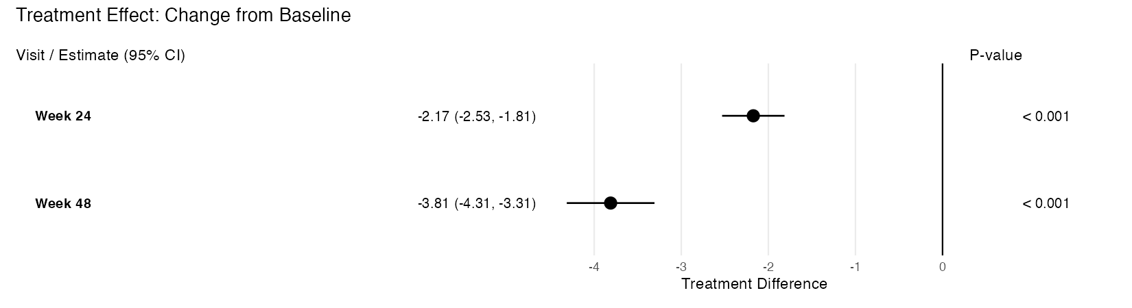
Create a Forest Plot from an rbmi Pool Object

Description

Takes an rbmi pool object and produces a publication-quality, three-panel forest plot using ggplot2 and patchwork. The plot displays treatment effect point estimates with confidence interval whiskers, an aligned table panel showing formatted estimates, and a p-value panel.

Usage

plot_forest(
  pool_obj,
  display = c("trt", "lsm"),
  ref_value = NULL,
  ci_level = NULL,
  arm_labels = NULL,
  title = NULL,
  text_size = 3.5,
  point_size = 3.5,
  show_pvalues = TRUE,
  font_family = NULL,
  panel_widths = NULL
)

Arguments

Details

The function calls tidy_pool_obj() internally to parse the pool object, then constructs a three-panel composition:

• Left panel: Visit labels and formatted estimate with CI text

• Middle panel: Forest plot with point estimates and CI whiskers

• Right panel: Formatted p-values

Display modes:

• "trt" – Treatment differences with a reference line at zero (or custom ref_value). Significant results (CI excludes reference) are shown as filled circles; non-significant as open circles.

• "lsm" – LS mean estimates by treatment arm, color-coded using the Okabe-Ito colorblind-friendly palette (blue for reference, vermilion for treatment). Points are dodged vertically within each visit.

Customization: The returned patchwork object supports ⁠& theme()⁠ for applying theme changes to all panels. For example: plot_forest(pool_obj) & theme(text = element_text(size = 14)).

Suggested dimensions for regulatory documents: For A4 or US Letter page sizes, ⁠width = 10, height = 3 + 0.4 * n_visits⁠ (in inches) provides good results when saving with ggplot2::ggsave(). For example, a 5-visit plot works well at 10 x 5 inches.

Example output (treatment difference mode):

Value

A patchwork/ggplot object that can be further customized using ⁠& theme()⁠ to modify all panels simultaneously.

See Also

• rbmi::pool() for creating pool objects

• tidy_pool_obj() for the underlying data transformation

• efficacy_table() for tabular presentation of the same data

• format_pvalue() for p-value formatting rules

• format_estimate() for estimate with CI formatting

Examples

if (requireNamespace("ggplot2", quietly = TRUE) &&
    requireNamespace("patchwork", quietly = TRUE)) {
  library(rbmi)
  data("ADMI", package = "rbmiUtils")
  ADMI$TRT <- factor(ADMI$TRT, levels = c("Placebo", "Drug A"))
  ADMI$USUBJID <- factor(ADMI$USUBJID)
  ADMI$AVISIT <- factor(ADMI$AVISIT)

  vars <- set_vars(
    subjid = "USUBJID", visit = "AVISIT", group = "TRT",
    outcome = "CHG", covariates = c("BASE", "STRATA", "REGION")
  )
  method <- method_bayes(
    n_samples = 20,
    control = control_bayes(warmup = 20, thin = 1)
  )

  ana_obj <- analyse_mi_data(ADMI, vars, method, fun = ancova)
  pool_obj <- pool(ana_obj)

  # Treatment difference forest plot
  plot_forest(pool_obj, arm_labels = c(ref = "Placebo", alt = "Drug A"))

  # LSM display with custom panel widths
  plot_forest(
    pool_obj,
    display = "lsm",
    arm_labels = c(ref = "Placebo", alt = "Drug A"),
    title = "LS Mean Estimates by Visit",
    panel_widths = c(3, 5, 1.5)
  )
}

Convert Pool Object to ARD Format

Description

Converts an rbmi pool object to the pharmaverse Analysis Results Dataset (ARD) standard using the cards package. The ARD format is a long-format data frame where each row represents a single statistic for a given parameter, with grouping columns for visit, parameter type, and least-squares-mean type.

Usage

pool_to_ard(pool_obj, analysis_obj = NULL, conf.level = NULL)

Arguments

Details

The function works by:

1. Tidying the pool object via tidy_pool_obj()

2. Reshaping each parameter into long-format ARD rows (one row per statistic)

3. Adding grouping columns (visit, parameter_type, lsm_type)

4. Optionally enriching with MI diagnostic statistics when analysis_obj is provided

5. Applying cards::as_card() and cards::tidy_ard_column_order() for standard ARD structure

When analysis_obj is provided:

• For Rubin's rules pooling: diagnostic statistics (FMI, lambda, RIV, Barnard-Rubin adjusted df, relative efficiency) are computed per parameter using the per-imputation estimates, standard errors, and degrees of freedom.

• For non-Rubin pooling methods: an informative message is emitted and the base ARD is returned without diagnostic rows.

The resulting ARD passes cards::check_ard_structure() validation and is suitable for downstream use with gtsummary.

Value

A data frame of class "card" (ARD format) with grouping columns for visit (group1), parameter_type (group2), and lsm_type (group3). Each parameter produces rows for five statistics: estimate, std.error, conf.low, conf.high, and p.value, plus a method row. When analysis_obj is provided and the pooling method is Rubin's rules, additional diagnostic stat rows are included: fmi, lambda, riv, df.adjusted, df.complete, re, and m.imputations.

See Also

• rbmi::pool() for creating pool objects

• analyse_mi_data() for creating analysis objects

• tidy_pool_obj() for the underlying data transformation

• cards::as_card() and cards::check_ard_structure() for ARD validation

Examples

if (requireNamespace("cards", quietly = TRUE)) {
  library(rbmi)
  data("ADMI", package = "rbmiUtils")
  ADMI$TRT <- factor(ADMI$TRT, levels = c("Placebo", "Drug A"))
  ADMI$USUBJID <- factor(ADMI$USUBJID)
  ADMI$AVISIT <- factor(ADMI$AVISIT)

  vars <- set_vars(
    subjid = "USUBJID", visit = "AVISIT", group = "TRT",
    outcome = "CHG", covariates = c("BASE", "STRATA", "REGION")
  )
  method <- method_bayes(
    n_samples = 20,
    control = control_bayes(warmup = 20, thin = 1)
  )

  ana_obj <- analyse_mi_data(ADMI, vars, method, fun = ancova)
  pool_obj <- pool(ana_obj)

  # Base ARD
  ard <- pool_to_ard(pool_obj)

  # Enriched ARD with MI diagnostics (FMI, lambda, RIV, df)
  ard_diag <- pool_to_ard(pool_obj, analysis_obj = ana_obj)
}

Prepare Intercurrent Event Data

Description

Builds a data_ice data.frame from a column in the dataset that flags intercurrent events. For each subject, the first visit (by factor level order) where the flag is TRUE is used as the ICE visit.

Usage

prepare_data_ice(data, vars, ice_col, strategy)

Arguments

Value

A data.frame with columns corresponding to vars$subjid, vars$visit, and vars$strategy, suitable for passing to rbmi::draws().

See Also

• rbmi::draws() which accepts the data_ice output from this function

• validate_data() to check data before imputation

• summarise_missingness() to understand missing data patterns

Examples

library(rbmi)

dat <- data.frame(
  USUBJID = factor(rep(c("S1", "S2", "S3"), each = 3)),
  AVISIT = factor(rep(c("Week 4", "Week 8", "Week 12"), 3),
                  levels = c("Week 4", "Week 8", "Week 12")),
  TRT = factor(rep(c("Placebo", "Drug A", "Drug A"), each = 3)),
  CHG = rnorm(9),
  DISCFL = c("N","N","N", "N","Y","Y", "N","N","Y")
)

vars <- set_vars(
  subjid = "USUBJID",
  visit = "AVISIT",
  group = "TRT",
  outcome = "CHG"
)

ice <- prepare_data_ice(dat, vars, ice_col = "DISCFL", strategy = "JR")
print(ice)

Print Method for Analysis Objects

Description

Prints a summary of an analysis object from analyse_mi_data().

Usage

## S3 method for class 'analysis'
print(x, ...)

Arguments

Value

Invisibly returns the input object.

Examples

library(rbmi)
library(rbmiUtils)
data("ADMI")

# Create analysis object
vars <- set_vars(
  subjid = "USUBJID", visit = "AVISIT", group = "TRT",
  outcome = "CHG", covariates = c("BASE", "STRATA")
)
method <- method_bayes(n_samples = 10, control = control_bayes(warmup = 10))

ana_obj <- analyse_mi_data(ADMI, vars, method, fun = function(d, v, ...) 1)
print(ana_obj)

Print Method for describe_draws Objects

Description

Displays a formatted summary of a draws description using cli formatting.

Usage

## S3 method for class 'describe_draws'
print(x, ...)

Arguments

Value

Invisibly returns x (for pipe chaining).

Examples

## Not run: 
# After creating draws_obj via the rbmi pipeline (see describe_draws):
desc <- describe_draws(draws_obj)
print(desc)  # Formatted cli output with method, formula, samples, convergence

## End(Not run)

Print Method for describe_imputation Objects

Description

Displays a formatted summary of an imputation description using cli formatting, including method, number of imputations, reference arm mappings, and a missingness breakdown by visit and treatment arm.

Usage

## S3 method for class 'describe_imputation'
print(x, ...)

Arguments

Value

Invisibly returns x (for pipe chaining).

Examples

## Not run: 
# After creating impute_obj via the rbmi pipeline (see describe_imputation):
desc <- describe_imputation(impute_obj)
print(desc)  # Formatted cli output with method, M, subjects, references, missingness

## End(Not run)

Print Method for Pool Objects

Description

Displays a formatted summary of a pooled analysis object from rbmi::pool(). Uses cli formatting to show rounded estimates, confidence intervals, parameter labels, method information, number of imputations, and confidence level.

Usage

## S3 method for class 'pool'
print(x, digits = 2, ...)

Arguments

Details

This method overrides rbmi::print.pool() to provide enhanced, formatted console output using the cli package. The override produces a "Registered S3 method overwritten" message at package load time, which is expected and harmless (same pattern as print.analysis()).

The output includes:

• A header with parameter and visit counts

• Metadata: pooling method, number of imputations, confidence level

• A compact results table with key columns: parameter, visit, est, lci, uci, pval

Value

Invisibly returns the original pool object x (for pipe chaining).

See Also

• tidy_pool_obj() for full tidy tibble output

• summary.pool() for visit-level breakdown with significance flags

• rbmi::pool() to create pool objects

Examples

library(rbmi)
library(rbmiUtils)
data("ADMI")

ADMI$TRT <- factor(ADMI$TRT, levels = c("Placebo", "Drug A"))
ADMI$USUBJID <- factor(ADMI$USUBJID)
ADMI$AVISIT <- factor(ADMI$AVISIT)

vars <- set_vars(
  subjid = "USUBJID", visit = "AVISIT", group = "TRT",
  outcome = "CHG", covariates = c("BASE", "STRATA", "REGION")
)
method <- method_bayes(n_samples = 20, control = control_bayes(warmup = 20))

ana_obj <- analyse_mi_data(ADMI, vars, method, fun = ancova)
pool_obj <- pool(ana_obj)
print(pool_obj)

Reduce Imputed Data for Efficient Storage

Description

Extracts only the imputed records (those that were originally missing) from a full imputed dataset. This significantly reduces storage requirements when working with many imputations, as observed values are identical across all imputations and only need to be stored once in the original data.

Usage

reduce_imputed_data(imputed_data, original_data, vars)

Arguments

Details

Storage savings depend on the proportion of missing data. For example:

• Original: 1000 rows, 44 missing values

• Full imputed (1000 imputations): 1,000,000 rows

• Reduced (1000 imputations): 44,000 rows (4.4\

Use expand_imputed_data() to reconstruct the full imputed dataset when needed for analysis.

Value

A data.frame containing only the rows from imputed_data that correspond to originally missing outcome values. All columns from imputed_data are preserved.

See Also

• rbmi::impute() which creates the imputed datasets this function operates on

• expand_imputed_data() to reconstruct the full dataset

• get_imputed_data() to extract imputed data from an rbmi imputation object

Examples

library(rbmi)
library(dplyr)

# Example with package data
data("ADMI", package = "rbmiUtils")
data("ADEFF", package = "rbmiUtils")

# Prepare original data to match ADMI structure
original <- ADEFF |>
  mutate(
    TRT = TRT01P,
    USUBJID = as.character(USUBJID)
  )

vars <- set_vars(
  subjid = "USUBJID",
  visit = "AVISIT",
  group = "TRT",
  outcome = "CHG"
)

# Reduce to only imputed values
reduced <- reduce_imputed_data(ADMI, original, vars)

# Compare sizes
cat("Full imputed rows:", nrow(ADMI), "\n")
cat("Reduced rows:", nrow(reduced), "\n")
cat("Compression:", round(100 * nrow(reduced) / nrow(ADMI), 1), "%\n")

Summarise Missing Data Patterns

Description

Tabulates missing outcome data by visit and treatment group, and classifies each subject's missing data pattern as complete, monotone, or intermittent.

Usage

summarise_missingness(data, vars)

Arguments

Value

A list with three components:

by_visit

A tibble with columns: visit, group, n, n_miss, pct_miss

patterns

A tibble with columns: subjid, group, pattern ("complete", "monotone", or "intermittent"), dropout_visit (NA if not monotone)

summary

A tibble with columns: group, n_subjects, n_complete, n_monotone, n_intermittent

See Also

• rbmi::draws() for imputation after reviewing missingness patterns

• validate_data() to check data before imputation

• prepare_data_ice() to create intercurrent event data from flags

Examples

library(rbmi)

dat <- data.frame(
  USUBJID = factor(rep(c("S1", "S2", "S3", "S4"), each = 3)),
  AVISIT = factor(rep(c("Week 4", "Week 8", "Week 12"), 4),
                  levels = c("Week 4", "Week 8", "Week 12")),
  TRT = factor(rep(c("Placebo", "Drug A"), each = 6)),
  CHG = c(1, 2, 3, 1, NA, NA, 1, 2, NA, 1, NA, 2)
)

vars <- set_vars(
  subjid = "USUBJID",
  visit = "AVISIT",
  group = "TRT",
  outcome = "CHG"
)

result <- summarise_missingness(dat, vars)
print(result$by_visit)
print(result$patterns)
print(result$summary)

Summary Method for Analysis Objects

Description

Provides a detailed summary of an analysis object from analyse_mi_data().

Usage

## S3 method for class 'analysis'
summary(object, n_preview = 5, ...)

Arguments

Value

A list containing summary information (invisibly).

Examples

library(rbmi)
library(rbmiUtils)
data("ADMI")

# Create analysis object
vars <- set_vars(
  subjid = "USUBJID", visit = "AVISIT", group = "TRT",
  outcome = "CHG", covariates = c("BASE", "STRATA")
)
method <- method_bayes(n_samples = 10, control = control_bayes(warmup = 10))

ana_obj <- analyse_mi_data(ADMI, vars, method, fun = function(d, v, ...) 1)
summary(ana_obj)

Summary Method for Pool Objects

Description

Provides a detailed visit-level breakdown of pooled analysis results with significance flags. Shows treatment comparisons and least squares means grouped by visit.

Usage

## S3 method for class 'pool'
summary(object, alpha = 0.05, ...)

Arguments

Details

The summary output groups results by visit, showing treatment comparisons with significance flags and least squares means. This provides a quick overview of which visits have statistically significant treatment effects.

Significance flags:

• * p < alpha (default 0.05)

• ⁠**⁠ p < 0.01

• ⁠***⁠ p < 0.001

Value

Invisibly returns a list with:

n_parameters

Number of parameters in the pool object

visits

Character vector of unique visit names

method

Pooling method used

n_imputations

Number of imputations combined

conf.level

Confidence level

tidy_df

The full tidy tibble from tidy_pool_obj()

See Also

• print.pool() for compact tabular output

• tidy_pool_obj() for full tidy tibble output

• rbmi::pool() to create pool objects

Examples

library(rbmi)
library(rbmiUtils)
data("ADMI")

ADMI$TRT <- factor(ADMI$TRT, levels = c("Placebo", "Drug A"))
ADMI$USUBJID <- factor(ADMI$USUBJID)
ADMI$AVISIT <- factor(ADMI$AVISIT)

vars <- set_vars(
  subjid = "USUBJID", visit = "AVISIT", group = "TRT",
  outcome = "CHG", covariates = c("BASE", "STRATA", "REGION")
)
method <- method_bayes(n_samples = 20, control = control_bayes(warmup = 20))

ana_obj <- analyse_mi_data(ADMI, vars, method, fun = ancova)
pool_obj <- pool(ana_obj)
summary(pool_obj)

Tidy and Annotate a Pooled Object for Publication

Description

This function processes a pooled analysis object of class pool into a tidy tibble format. It adds contextual information, such as whether a parameter is a treatment comparison or a least squares mean, dynamically identifies visit names from the parameter column, and provides additional columns for parameter type, least squares mean type, and visit.

Usage

tidy_pool_obj(pool_obj)

Arguments

Details

The function dynamically processes the parameter column by separating it into components (e.g., type of estimate, reference vs. alternative arm, and visit), and provides informative descriptions in the output.

Workflow:

1. Prepare data and run imputation with rbmi

2. Analyse with analyse_mi_data()

3. Pool with rbmi::pool()

4. Tidy with tidy_pool_obj() for publication-ready output

Value

A tibble containing the processed pooled analysis results with the following columns:

parameter

Original parameter name from the pooled object

description

Human-readable description of the parameter

visit

Visit name extracted from parameter (if applicable)

parameter_type

Either "trt" (treatment comparison) or "lsm" (least squares mean)

lsm_type

For LSM parameters: "ref" (reference) or "alt" (alternative)

est

Point estimate

se

Standard error

lci

Lower confidence interval

uci

Upper confidence interval

pval

P-value

See Also

• rbmi::pool() which creates the pool objects this function tidies

• analyse_mi_data() to analyse imputed datasets

• format_results() for additional formatting options

Examples

# Example usage:
library(dplyr)
library(rbmi)

data("ADMI")
N_IMPUTATIONS <- 100
BURN_IN <- 200
BURN_BETWEEN <- 5

# Convert key columns to factors
ADMI$TRT <- factor(ADMI$TRT, levels = c("Placebo", "Drug A"))
ADMI$USUBJID <- factor(ADMI$USUBJID)
ADMI$AVISIT <- factor(ADMI$AVISIT)

# Define key variables for ANCOVA analysis
 vars <- set_vars(
  subjid = "USUBJID",
  visit = "AVISIT",
  group = "TRT",
  outcome = "CHG",
  covariates = c("BASE", "STRATA", "REGION")  # Covariates for adjustment
 )

# Specify the imputation method (Bayesian) - need for pool step
method <- rbmi::method_bayes(
  n_samples = N_IMPUTATIONS,
  control = rbmi::control_bayes(
    warmup = BURN_IN,
    thin = BURN_BETWEEN
    )
  )

# Perform ANCOVA Analysis on Each Imputed Dataset
ana_obj_ancova <- analyse_mi_data(
  data = ADMI,
  vars = vars,
  method = method,
  fun = ancova,  # Apply ANCOVA
  delta = NULL   # No sensitivity analysis adjustment
)

pool_obj_ancova <- pool(ana_obj_ancova)
tidy_df <- tidy_pool_obj(pool_obj_ancova)

# Print tidy data frames
print(tidy_df)

Validate Data Before Imputation

Description

Pre-flight validation of data, variable specification, and intercurrent event data before calling rbmi::draws(). Collects all issues and reports them together in a single error message.

Usage

validate_data(data, vars, data_ice = NULL)

Arguments

Details

The following checks are performed:

• data is a data.frame

• All columns named in vars exist in data

• subjid, visit, and group columns are factors

• outcome column is numeric

• Covariate columns have no missing values

• Data has one row per subject-visit combination

• If data_ice is provided: correct columns, valid subjects, valid visits, recognised strategies, and at most one row per subject

Recommended Workflow:

1. Call validate_data() to check your data

2. Use prepare_data_ice() to create ICE data if needed

3. Review missingness with summarise_missingness()

4. Proceed with rbmi::draws() for imputation

Value

Invisibly returns TRUE if all checks pass. Throws an error with collected messages if any issues are found.

See Also

• rbmi::draws() which requires validated input data

• prepare_data_ice() to create intercurrent event data from flags

• summarise_missingness() to understand missing data patterns

Examples

library(rbmi)

dat <- data.frame(
  USUBJID = factor(rep(c("S1", "S2", "S3"), each = 3)),
  AVISIT = factor(rep(c("Week 4", "Week 8", "Week 12"), 3),
                  levels = c("Week 4", "Week 8", "Week 12")),
  TRT = factor(rep(c("Placebo", "Drug A", "Drug A"), each = 3)),
  CHG = c(1.1, 2.2, 3.3, 0.5, NA, NA, 1.0, 2.0, NA),
  BASE = rep(c(10, 12, 11), each = 3),
  STRATA = factor(rep(c("A", "B", "A"), each = 3))
)

vars <- set_vars(
  subjid = "USUBJID",
  visit = "AVISIT",
  group = "TRT",
  outcome = "CHG",
  covariates = c("BASE", "STRATA")
)

validate_data(dat, vars)